P = NP can be proven?

I have a hunch that P=NP can actually be proven.

It is known that in this chain of inclusions:
$$ P \subseteq NP \subseteq PSPACE \subseteq EXPTIME $$ at least one inclusion is proper (ie, equality does not hold), by the "Time Hierarchy theorem". Other than that, none of the inclusions have been proven to be proper so far. Note that this theorem is proved via diagonalization, ie, Cantor's theorem that the cardinality of a power set must be bigger than the cardinality of the set itself. In other words, the proof is based on cardinality. But (with my limited knowledge and saying this vaguely) I have not known of similar cardinality proofs that are "smaller" than Cantor's. Does it mean that there is only 1 inequality within that chain?

What is Montague grammar?

Montague grammar

Richard Montague developed his theory of grammar from 1950-1970s.  What is special about Montague grammar is that, whereas Chomsky's transformational grammar provides a formal account for the syntax of natural language, Montague grammar has both formal syntax and semantics.

Basically, Montague uses categorial grammar to describe the syntax of a natural language.  Then he establishes formal translation rules that maps natural-language sentences to logical formulas in intensional logic.  Such formulas have well-defined semantics based on possible worlds.

Let's turn to the semantics first, since it is the most interesting and relevant to AGI...

Intensional logic (內涵邏輯)

Intensional logic originated as an attempt to resolve paradoxes due to confusing references with senses (指涉 和 涵義), or extensions with intensions (外延 和 內涵).  Its idea has been studied by Frege (1892), Lewis (1914), Tarski (1933), Carnap (1947), Kripke (1963), Montague (1970).

To say that:
       The Empire State Building is the tallest building in New York
is not the same as saying:
       The tallest building in New York is the tallest building in New York
even though we have substituted equal by equal.  How come?

The problem is that "the tallest building in New York" is a symbol that has a reference (or extension) which is the object it refers to, and a sense (or intension) which is more subtle and depends on the context under which it is interpreted.

In different possible worlds (such as different time periods), "the tallest building in New York" can refer to different objects.  While the extension of a symbol can be taken as the set of individuals it refers to, the intension of the symbol cannot be such a set, but has to be the function that maps from possible worlds to individuals in the worlds.  As shown in the diagram:

In other words, the function associates to each possible world an individual in that world which the symbol refers to.  That is:

$ f: I \rightarrow U $

$ f: i \mapsto u $

where $I$ is the set of possible worlds (or interpretations), and $U$ is the set of individuals that figure in any of the worlds.

The intensional logic (IL) as described by Montague is a meta-language based on $\lambda$-calculus, that allows to define various modal operators, so that it can subsume modal logic, temporal logic, deontic logic, and epistemic logic, etc.

Compound nouns

I discovered that intension functions may also help us define the semantics of compound nouns, such as:

cyber sex	sex that happens on the internet
glass slippers	slippers made of glass
couch potato	person who stays in the couch all the time

Some compound nouns are easy to interpret as they are simply the conjunction of their constituent atomic concepts.  For example, a "girl scout" is both a "girl" and a "scout".  However, a "girl school" is not a "girl", but is for girls.  The meaning of such atypical compound nouns seem to require abductive interpretation (溯因解釋).  Abduction means to search for explanations for what is known, which is the reverse of deduction which searches from what is known to new conclusions.

Now with the insight from intensional logic, perhaps we can interpret compound nouns like this:

So each modifier is a function that maps from possible worlds to individuals.

The advantage of such a treatment is that concept composition in general can be uniformly represented by intensional logic.

What is a function?

When we say "there exists a function...", it can be deceptive as the function can be any arbitrary mapping -- for example, it can include a bizarre map that maps an individual to Confucius in world$_1$, to the number 7 in world$_2$, to the Empire State Building in world$_3$, etc.  What we need is to operationalize the concept of functions.

In the logic-based paradigm, a function is implemented as a set of logic formulas that determine the elements of a predicate.  For example, the Prolog program:
    ancestor(X,Y) :- father(X,Y)
    ancestor(X,Y) :- ancestor(X,Z), father(Z,Y)
    etc...
determines the elements of the "ancestor" relation.

So we have found an operational implementation for functions, and as logic programs are Turing universal, they are also the broadest class of functions we can define.  One question is whether we can simplify the logical form, while keeping its Turing universality.

Possible world semantics

Possible world semantics were developed by Carnap and Kripke, among others, but Leibniz was the first "logician" to use the term "possible world".

The relevance to intensional logic is that each intensional individual is a function from the set of possible worlds (W) to the set of possible individuals (D):
    $ f : W \rightarrow D $.
In other words, the set of all intensional individuals is $D^W$.

Possible world semantics is a way to model modal logics (模態邏輯).  Modal logic is distinguished by the use of the modal operators $\Box$ "necessarily" and $\diamond$ "possibly".  To model a logic means to establish a correspondence between propositions (命題) in the logic and an underlying algebraic structure called interpretations, such that the truth of propositions in the logic can be determined (or evaluated) by looking into that algebraic structure.  In the case of modal logic, its model can be given by Kripke structures, or possible worlds.

What is a Kripke structure?  It is a tuple $\left< W, R, V \right>$ of possible worlds $W$, a binary accessibility relation $R$ between worlds, and a valuation map $V$ assigning {true, false} to each proposition $p$ in possible world $w$.

Modal truths are defined by this interpretation rule:
     $ \Box \phi \Leftrightarrow \forall w \in W. \phi $
which means that $\phi$ is necessarily true, if $\phi$ is true in all possible worlds in $W$.  There is also a dual rule for $\diamond$.

This is an example Kripke structure:

Where the $w$'s are possible worlds, with $w_0$ being a distinguished "current state" or "real world", the arrows are "reachable" relations, and the $a, b$'s are propositions true in those worlds.  This example may model a computational process, where we want to ensure, say, "state 0 will never be reached after N steps".  Such a statement can be translated into modal logic and be verified by a model checker.  This debugging technique is what enables the design of highly complex modern microprocessors.

Categorial grammar

{ For completeness' sake ... }

References:

[1] Portner 2005.  What is meaning? - fundamentals of formal semantics.  Blackwell Publishing.

[2] James McCawley 1993.  Everything that linguists have always wanted to know about logic *but were ashamed to ask, 2nd ed.  Chicago.

[3] 朱水林 1992 (ed). 邏輯語義學研究 (Studies in logical semantics)。上海教育出版社

[4] 鄒崇理 2000.  自然語言研究 (Natural language linguistics)。北京大學出版社

[5] 陳道德 2007 (ed).  二十世紀意義理論的發展與語言邏輯的興起 (20th century semantic theory and the rise of logical linguistics)。 北京社會科學出版社

[6] 方立 2000.  邏輯語義學 (Logical semantics: an introduction)。  北京語言文化大學出版社

[7] J v Benthem 2010.  Modal logic for open minds.  CSLI publications

[8] Gopalakrishnan 2006.  Computation engineering - applied automata theory and logic.  Springer.

Mathematics behind Google's page rank algorithm

Thanks to professor Raymond Chan of CUHK mathematics, who gave an undergrad talk on the mathematics of Google, which I attended by chance.  In this post I'll try to re-present what he said, with some of my own variations.  (Mistakes, if any, are mine.)

I also combined materials from chapter 2 of the book "A First Course in Applied Mathematics" by Jorge Rebaza (2012):

How much is the PageRank algorithm worth?

In 2012:
    Google annual revenue = US 50.2   billion
    Google total assets        = US 93.8   billion
    Google market cap        = US 248.2 billion
    Hong Kong's GDP         = US 243.7 billion

So the entire Hong Kong population working for a year, is roughly worth the outstanding stocks of Google.  Perhaps learning the PageRank algorithm can give us an estimate of how useful mathematics can be :)

The algorithm

As of 2012 Google is searching 8.9 billion web pages.  First, it builds a directed graph ($\Gamma$) of how the web pages are linked to each other.

Example 1:

$$ A = \left[ \begin{array}{c c c c c} 0 & 0 & 0 & 1 & 0 \\  0 & 0 & 0 & 0 & 1 \\  0 & 1/2 & 0 & 0 & 1/2 \\ 1 & 0 & 0 & 0 & 0 \\  0 & 1 & 0 & 0 & 0  \end{array}  \right] $$

Example 2:

$$ A = \left[ \begin{array}{c c c c c c} 0 & 1 & 0 & 0 & 0 & 0 \\  1/2 & 0 & 1/2 & 0 & 0 & 0 \\  1/2 & 1/2 & 0 & 0 & 0 & 0 \\ 0 & 0 & 1/3 & 0 & 1/3 & 1/3 \\  0 & 0 & 0 & 0 & 0 & 0 \\ 0 & 0 & 0 & 1/2 & 1/2 & 0 \end{array}  \right] $$

In the graph:
    nodes = web pages
    links   = out-going links from page to page

The matrices are the adjacency matrices of the graphs.  Each row represents the out-going links from the page $P_i$.  If a page has $n$ out-going links, each link is weighted by $1/n$.

Notice that each row of the matrices sum to 1.  These are called stochastic matrices.

Then the rank of a page is defined by adding up the ranks of pages with out-links pointing to it:

$$  r(P) = \sum_{i} \frac{r(P_i)}{|P_i|} $$
where $r(P_i)$ is the rank of Page $i$, and $|P_i|$ denotes the total number of out-going links from Page $i$.  The rationale is that it is a good thing to be pointed to, so the "goodness" of Page $i$ is passed to Page $P$;  but it has to be divided by $|P_i|$ because a page that points outwards "promiscuously" should have its influence diluted.

But this ranking has to be calculated iteratively starting from an initial ranking.  The iterative equation has the form:
$$ r_k(P) = \sum_i \frac{r_{k-1}(P_i)}{|P_i|}, \quad \quad k = 1, 2, ... $$

This means that the "goodness" (ranking) is passed around the graph iteratively until their values at every node converge to stable values.

In vector notation:  let $v_k = [ r_k(P_1) \; r_k(P_2) \; ... \; r_k(P_N) ]^T $.  Then the iterative equation becomes:
$$ v^T_k = v^T_{k-1} H $$
where
$$ H_{ij} = \left\{ \begin{array}{l@l} \frac{1}{|P_i|} & \mbox{if } P_i \mbox{ has a link to } P \\ 0 & \mbox{otherwise} \end{array} \right. $$

Notice that matrix H is constant throughout the iteration.  That means we are repeatedly multiplying by H:
$$ v = \lim_{k \rightarrow \infty} v_k = \lim_{k \rightarrow \infty} H^k v_0 $$
where $v$ is the PageRank vector.

The above is reminiscent of the way we repeatedly press the "cosine" button on a calculator, and see the results converge.  That value is the solution to the equation:
$$ \cos x = x. $$
In general, when we want to solve an equation of the form $ f(x) = x $, we can repeatedly apply $f()$ starting from an initial value $x_0$.  The point for which $f(x^*) = x^*$ is called the fixed point, a very useful concept in mathematics.

The above iteration is called the power method, which will converge to the eigenvector with the greatest eigenvalue of the matrix $H$.  This is called the dominant eigenvector, which I will now explain...

Power method

This section explains why the power method converges.  Recall the definition of eigenvector and eigenvalue:
$$ A x = \lambda x $$
where $x$ = eigenvector, $\lambda$ = eigenvalue.

Assume that the matrix A satisfies these conditions:

• $A$ has a complete set of linearly independent eigenvectors $v_1, ... v_n$
• the corresponding eigenvalues can be ordered:
                $ |\lambda_1| > |\lambda_2| \ge ... \ge |\lambda_n| $
  (notice the strict > in the first term)

For iteration, choose an arbitrary initial vector $x_0$.  Due to the eigenvectors forming a basis, we can express $x_0$ as:

$$ x_0 = c_1 v_1 + ... + c_n v_n $$

Now we multiply the above with matrix A and get:

$$ \begin{array}{l@=l} A x_0 & = c_1 \lambda_1 v_1 + c_2 \lambda_2 v_2 + ... + c_n \lambda_n v_n \\ A^2 x_0 & = c_1 \lambda_1^2 v_1 + c_2 \lambda_2^2 v_2 + ... + c_n \lambda_n^2 v_n \\ & \vdots \\ A^k x_0 & = c_1 \lambda_1^k v_1 + c_2 \lambda_2^k v_2 + ... + c_n \lambda_n^k v_n \end{array} $$

And because $ |\lambda_1| > |\lambda_2| \ge ... \ge |\lambda_n| $, as $k \rightarrow \infty$, the weight of the first term outgrows those of the rest, so the vector $A^k x_0$ moves towards the dominant eigenvector direction.

The rate of convergence is determined by the ratio $\frac{ |\lambda_2| } { |\lambda_1| }$.

For the power method to converge, we need to ensure that the matrix is stochastic and irreducible....

Irreducible matrices

The section explains the necessary condition for the power method to converge;  but the measure to force convergence also gave rise to Google's personalized search, as we shall see why.

A matrix is called reducible if there exists a permutation matrix $P$ such that:
$$ P^T A P = \left[ \begin{array}{cc} C& D \\ \mathbf{0} & E \end{array} \right] $$
where $\mathbf{0}$ is a $(n-r) \times r$ block matrix with 0's.

Observe that the above definition expresses the similarity between $A$ and a block upper triangular matrix.  (Note:  2 matrices $A$ and $B$ are similar if there is a $P$ such that $B = P A P^{-1}$, where P is any invertible matrix.  This means that the effect of applying $A$ is the same as applying $B$ between a change of coordinates and back.  In the case of permutation matrices, $P^{-1}$ coincides with $P^T$.)

The significance of this definition is that:

matrix A is irreducible $\Longleftrightarrow \Gamma(A) $ is strongly connected

A graph is strongly connected if every node is reachable from any other node.

Example:

where
$$ A = \left[ \begin{array}{c c c c} 0 & 1/3 & 1/3 & 1/ 3 \\ 1/2 & 0 & 1/2 & 0 \\ 0 & 0 & 0 & 1 \\ 0 & 0 & 1 & 0 \end{array} \right] $$


$$ B = \left[ \begin{array}{c c c c} 0 & 1 & 0 & 0 \\ 1 & 0 & 0 & 0 \\ 1/3 & 1/3 & 0 & 1/3 \\ 1/2 & 0 & 1/2 & 0  \end{array} \right] $$

$$ B = P^T A P $$ 

$$ P = \left[ \begin{array}{c c c c} 0 & 0 & 1 & 0 \\ 0 & 0 & 0 & 1 \\ 1 & 0 & 0 & 0 \\ 0 & 1 & 0 & 0  \end{array} \right] $$

The effect of multiplying by $P$ (a permutation matrix), is to exchange some rows, hence the name.
Notice that there is no way in matrix $A$ to go from the nodes 3 & 4 to nodes 1 & 2.  Thus matrix $A$ is reducible.

To ensure irreducibility (in order for the power method to work), Google forces every page to be reachable from every other page.

Google's solution is to add a perturbation matrix to $H$:

$$ G = \alpha H + (1 - \alpha) E  $$

where $G$ is the Google matrix, $\alpha \in (0,1)$, and $E = e \; e^T / n$ where $e$ is a vector or 1's.  This makes every page reachable to every page, but later Google modified this to:

$$ E = e \; u^T $$

where $u$ is a probabilistic vector called the personalization vector, which plays a great role in Google's success.  More details are explained in Rebaza's book.

Hope this is helpful to you :)

On visual recognition

I will try to consider visual recognition from a high level, though my approach may not be the only possible one.

We're given the image projected on the retina.  We seek the model that generated the image.  A mathematics-favored way is to think of the model as finitely generated from a set of primitives.  (The primitives could be infinite too, but let's start with simpler.)

For example, the primitives could be a class of geometric shapes such as cylinders, rectangles, polygons, etc.  These can be given concisely by their positions and size / shape parameters.

Bayesian learning

We are interested in finding the maximum of  $P(model | data)$, ie, the most probable model given the data.  The models would be specified by some parameters as model$(r)$.

Bayes' law says that:

$$P(model | data) = \frac{P(data | model) P(model)}{P(data)}.$$

What is special about this formula is that the right hand side contains $P(data | model)$ which is usually much easier to compute than the left hand side.

In our vision example, $P(data | model)$ means that we are given the model, so we can use the known function $f$ (see above figure) to compute the data.  Whereas, $P(model | data)$ requires us to use $f^{-1}$ to compute the model which is much harder.

But I have not spelled out the details of the computation, particularly at the pixel level...

A highly abstract and simple example

Now let's try to understand the whole process from an abstract perspective (without reference to Bayesian learning).

To reduce matters to the simplest case, let's consider recognizing straight lines on a $100 \times 100$ image (with noise).  Assume the input image always contains only 1 line, that could be slightly non-straight.

Every straight line can be represented by 2 parameters $(c,d)$ via its equation:

$ cx + dx = 1. $

So a naive, but impractical, algorithm is simply to:

• visit all points in the parameter space $(c,d)$
• draw each line as image data, $D$
• compare $D$ with our input image $D_0$
• return the line that minimizes the difference $\Delta(D, D_0)$

But of course, this is unfeasible because the search space $(c,d)$ is too large (indeed infinite).

Feature extraction

Vision researchers usually use a pre-processing stage known as feature extraction.  I'm not saying it is necessary, but let's see what happens.  The input image can be broken into a smaller number of edgels.  Their number is vastly smaller than the number of pixels.  Say, each edgel is 5 pixels long.  So a line across a $100 \times 100$ image would be on the order of ~20 edgels long.

The situation can be summarized by this commutative diagram:

We know how to do $f$, which we assume is easy.  And assume we know how to do $\Phi$.  So we know how to do $\Psi = \Phi \circ f$.

Now instead of computing the error with the raw image:

$\Delta_1 = || f(\mathbf{r}) - D_0 || $

we can compare their features-space representations:

$\Delta_2 = || \Psi(\mathbf{r}) - \Phi(D_0) || $

which is more efficient (maybe?).

For our example, we can use $(c,d)$ to generate a set of features $F$, which are edgels each having a position and slope.  In symbols:

$(c,d) \stackrel{\Psi}{\mapsto} F = \bigcup_{i=1}^N \{ (x_i, y_i, slope_i) \} $

where the x, y and slopes are simple functions of the parameters $\mathbf{r} = (c,d)$.  The error could be defined as some kind of average of differences between individual edgel-pairs.

Notice that $\Psi^{-1}$ may still be difficult to compute.

See, the biggest inefficiency is actually not $\Psi$ itself, but is the size of the parameter space $(c,d)$, which forces us to evaluate $\Psi$ many times in a generate-and-test loop.

We can also see that feature extraction does not directly attack the bottleneck.

It would be very nice if we can directly calculate $\Psi^{-1}$.  Then we can simply go from the input data $D_0$ via $\Phi$ and $\Psi^{-1}$ to get our answer, $(c,d)$.  That does not require any searching!  How can that be done?

Two possible strategies

In fact we have 2 possible strategies:

• Along every step of the generative process $f$ or $\Psi$, use only invertible functions.
• Use only differentiable functions in every step, so then we can set $\frac{\partial \Delta}{\partial r} = 0$ and so on to find the minimum of the error.

In both strategies, we are writing a functional program using a restricted class of functions.  Then the computer can automatically find the inverse or derivatives for us, either numerically or symbolically.

In the first strategy, notice that some commonly-used functions do not have inverses.  In particular, if the function is idempotent (ie, $f \circ f = f$), which includes min, max, projection, and set union. Note however, that these functions may be invertible if we allow interval-valued or set-valued functions.  (Indeed, in vision we generally accept that one cannot see behind opaque objects, a consequence of the idempotency of occlusion.)

In the second strategy, we may need to create "soft" versions of non-differentiable functions such as min, max, and projection.

These are still rather vague, but I think are promising directions...

What about AI?

A final word is that we are just recognizing images as models composed of geometric primitives (such as cylinders).  That is still different from natural labels such as "hands", "trees", "cars", or even descriptions such as "nude descending a staircase".

For the latter purpose, we need a further map, say $\Theta$, from natural-language descriptions to geometric models:

I have an impression that this map $\Theta$ is best represented using logical form.  That is because many natural concepts, such as "chairs", do not have representations as connected regions in geometric space.  Rather, they are defined via complex and intricate, "intensional" relationships.  In other words, logical or relational.  The formalism I'm developing is somewhat like logic, somewhat like algebra, and a bit like neurons.  One can think of it as a universal language for expressing patterns in general.

Matrix trick and the ontology ball

Genifer's logic has the structure of a semi-ring obeying:

$\mbox{associative addition:} \quad (A + B) + C = A + (B + C) $

$\mbox{associative multiplication:} \quad (A \times B) \times C = A \times (B \times C) $

$\mbox{non-commutative multiplication:} \quad A \times B \neq B \times A $

$\mbox{distribution on the right}\quad (A + B) \times C = A \times C + B \times C $

$\mbox{commutative addition:} \quad A + B = B + A $

$\mbox{idempotent addition:} \quad A + A = A $

In short, multiplication is similar to "concatenation of letters" and addition is like "set union".  In programming (data-structure) terms, the algebra is like a set of strings composed of letters, and the letters are what I call concepts.

Matrix trick

The matrix trick is simply to represent the elements of the algebra by matrices.  (This may be related to representation theory in abstract algebra).

What is a matrix?  A matrix is a linear transformation.  For example, this is an original image:

This is the image after a matrix multiplication:

In short, matrix multiplication is equivalent to a combination of rotation, reflection, and/or shear.  You can play with this web app to understand it intuitively.

So my trick is to represent each concept, say "love", by a matrix.  Then a sentence such as "John loves Mary" would be represented by the matrix product "john $\otimes$ loves $\otimes$ mary".

Each arrow represents a matrix multiplication.  The transformations need not occur on the same plane.

By embedding the matrices in a vector space (simply writing the matrix entries as a flat vector), I can "locate" any sentence in the vector space, or cognitive space.

Keep in mind that the rationale for using matrices is solely because $AB \neq BA$ in matrix multiplication, or:

John loves Mary $\neq$ Mary loves John.

Ontology ball

This is another trick I invented:

It is just a representation of an ontology in space (as a ball).  To determine if $A \subset B$, we see if $A$ is located within the "light cone" of $B$.  Note that fuzzy $\in$ and $\subset$ can be represented by using the deviation from the central axis as a fuzzy measure.

I think this trick is important since it replaces the operation of unification (as in Prolog or first-order logic) with something spatial.  Traditionally, unification is done by comparing 2 logic terms syntactically, via a recursive-descent algorithm on their syntax trees.  This algorithm is discrete.  With this trick we can now perform the same operation using spatial techniques, which is potentially amenable to statistical learning.

Update:  Unfortunately I realized that the light-cone trick is not compatible with the matrix trick, as the matrix multiplication rotates the space which may destroy the $\in$ or $\subset$ relations (as they rely on straight rays projecting from the origin to infinity).  In fact, a matrix multiplication can be seen as a rotation of an angle $\theta$ which can expressed as a rational multiple of $\pi$ (or arbitrarily close if irrational).  Then we can always find a $k$ such that $A^k = Id$ where $Id$ is the identity.  In other words, we can find a product of any word, say "love", such that:

love $\circ$ love $\circ$ love ... = $Id$

which doesn't make sense.

I am still thinking of how to combine the 2 tricks.  If successful, it may enable us to perform logic inference in a spatial setting.  

Support vector machines

The 3 parts of an SVM

The SVM consists of 3 "tricks" combined to give one of the most influential and arguably state-of-the-art machine learning algorithm.  The 3rd, "kernel trick" is what gives SVM its power.

During the talk I will refer to Cortes and Vepnik's 1995 paper.

1. A linear classification problem, ie, separating a set of data points by a straight line / plane.  This is very simple.
2. Transforming the primal optimization problem to its dual via Lagrangian multipliers.  This is a standard trick that does not result in any gain / loss in problem complexity.  But the dual form has the advantage of depending only on the inner product of input values.
3. The kernel trick that transforms the input space to a high dimensional feature space.  The transform function can be non-linear and highly complex, but it is defined implicitly by the inner product.

1. The maximum-margin classifier

The margin is the separation between these 2 hyper-planes:

 $ \bar{w}^* \cdot \bar{x} = b^* + k $

 $ \bar{w}^* \cdot \bar{x} = b^* - k $

so the maximum margin is given by:

 $ m^* = \frac{2k}{|| \bar{w}^* ||} $

The optimization problem is to maximize $m^*$, which is equivalent to minimizing:
$$ \max (m^*) \Rightarrow \max_{\bar{w}} (\frac{2k}{ || \bar{w} || })
\Rightarrow \min_{\bar{w}} (\frac{ || \bar{w} || }{2k})  \Rightarrow \min_{\bar{w}} ( \frac{1}{2} \bar{w} \cdot \bar{w} ) $$subject to the constraints that the the hyper-plane separates the + and - data points:
$$ \bar{w} \cdot (y_i \bar{x_i} ) \ge 1 + y_i b $$

This is a convex optimization problem because the objective function has a nice quadratic form $\bar{w} \cdot \bar{w} = \sum \bar{w_i}^2$ which has a convex shape:

2. The Lagrangian dual

The Lagrangian dual of the maximum-margin classifier is to maximize:
$$ \max_{\bar{\alpha}} ( \sum_{i=1}^{l} \alpha_i - \frac{1}{2} \sum_{i=1}^{l} \sum_{j=1}^{l} \alpha_i \alpha_j y_i y_j \bar{x_i} \cdot \bar{x_j} ) $$subject to the constraints:
$$ \sum_{i=1}^l \alpha_i y_i = 0, \quad  \alpha_i \ge 0 $$
Lagrangian multipliers is a standard technique so I'll not explain it here.

Question:  why does the inner product appear in the dual?  But the important point is that the dual form is dependent only on this inner product $(\bar{x_i} \cdot \bar{x_j})$, whereas the primal form is dependent on $(\bar{w} \cdot \bar{w})$.  This allows us to apply the kernel trick to the dual form.

3. The kernel trick

A kernel is just a symmetric inner product defined as:
$$ k(\mathbf{x}, \mathbf{y}) = \Phi(\mathbf{x}) \cdot \Phi(\mathbf{y}) $$By letting $\Phi$ free we can define the kernel as we like, for example, $ k(\mathbf{x}, \mathbf{y}) = \Phi(\mathbf{x}) \cdot \Phi(\mathbf{y}) = (\mathbf{x} \cdot \mathbf{y} )^2 $.

In the Lagrangian dual, the dot product $(\bar{x_i} \cdot \bar{x_j})$ appears, which can be replaced by the kernel $k(\bar{x_i}, \bar{x_j}) = (\Phi(\bar{x_i}) \cdot \Phi(\bar{x_j}))$.

Doing so has the effect of transforming the input space $\mathbf{x}$ into a feature space $\Phi(\mathbf{x})$, as shown in the diagram:

But notice that $\Phi$ is not explicitly defined;  it is defined via the kernel, as an inner product.  In fact, $\Phi$ is not uniquely determined by a kernel function.

This is a possible transformation function $\Phi$ for our example:
$$ \Phi(\mathbf{x}) = (x_1^2, x_2^2, \sqrt{2} x_1 x_2) $$It just makes $ \Phi(\mathbf{x}) \cdot \Phi(\mathbf{y}) $ equal to $ (\mathbf{x} \cdot \mathbf{y} )^2 $.

Recall that the inner product induces a norm via:

$ ||\mathbf{x}|| = \sqrt{\mathbf{x} \cdot \mathbf{x}} $

and the distance between 2 points x and y can be expressed as:

$ d(\mathbf{x},\mathbf{y})^2 = || \mathbf{x - y} ||^2 = \mathbf{x} \cdot \mathbf{x} + \mathbf{y} \cdot \mathbf{y} - 2 \mathbf{x} \cdot \mathbf{y}$

Thus, defining the inner product is akin to re-defining the distances between data points, effectively "warping" the input space into a feature space with a different geometry.

Some questions:  What determines the dimension of the feature space?  How is the decision surface determined by the parameters $\alpha_i$?

Hilbert Space

A Hilbert space is just a vector space endowed with an inner product or dot product, notation $\langle \mathbf{x},\mathbf{y}\rangle$ or $(\mathbf{x} \cdot \mathbf{y})$.

The Hilbert-Schmidt theorem (used in equation (35) in the Cortes-Vapnik paper) says that every self-adjoint operator in a Hilbert space H (which can be infinite-dimensional) forms an orthogonal basis of H.  In other words, every vector in space H has a unique representation of the form:

$$ \mathbf{x} = \sum_{i=1}^\infty \alpha_i \mathbf{u}_i $$This is called a spectral decomposition.

*  *  *

As a digression, Hilbert spaces can be used to define function spaces.  For example, this is the graph of a function with an integer domain:

with values of $f(1), f(2), f(3), ... $ on to infinity.  So, each graph corresponds to one function.

Imagine an infinite dimensional space.  Each point in such a space has dimensions or coordinates $(x_1, x_2, ... )$ up to infinity.  So we can say that each point defines a function via
$$f(1) = x_1, \quad f(2) = x_2, \quad f(3) = x_3, ... $$
In other words, each point corresponds to one function.  That is the idea of a function space.  We can generalize from the integer domain ($\aleph_0$) to the continuum ($2^{\aleph_0}$), thus getting the function space of continuous functions.

End of digression :)

Introducing Genifer, 2012

I started working on AGI in 2004, and my greatest "achievement" up to 2012 (8 years) is the invention of a new logic.  All my work thus far is focused on the thinking aspect of AGI, deferring the aspects of planning and acting.

Concept composition logic

Consider a complex sentence:
     "John walks to church slowly, thinking about Turing"

It can be decomposed into:

1. "John walks to church"
2. "John walks slowly"
3. "John walks thinking about Turing"

Using the Genifer GUI (github code is here) we can manually create a graph that represent the sentence structure as follows:

The GUI automatically generates a "factorization" formula of the graph.

The key idea of the graph is that if a word A modifies word B, we create an arrow $A \multimap B$.  More than 1 word can modify a target, but each word can only modify 1 target.  This ensures that the result is a tree, and can be expressed as a sum of products, using $+$ and $\times$.

We can use the distributive law of multiplication to expand the factorized formula.

A problematic case:  If we translate these 2 sentences into logic:

1. "John gives the ball to Mary"  and
2. "John gives $2 to Kevin"

After factorizing and expanding we get:

1. john gives to mary
2. john gives the ball
3. john gives to kevin
4. john gives $2

so it may be confused that John gives $2 to Mary.  But I reckon that the distributive law is not the real cause of the error.  The error arises because the 2 "johns" are the same John but the 2 "gives" are different instances of giving.

Variable-free logic

This is an example of the logical definition of "downstairs" from the SUMO ontology:

On the left side is the logic formula, on the right the English translation.  As you can see from the translation, it uses a lot of "$n^{th}$ objects" which are logic variables.  But notice that all these variables invariably belong to some classes (such as "building_level").  So we can just do without variables and directly use ontology classes for matching.

For example:
    "All girls like to dress pretty"
    "Jane is a girl"
implies "Jane likes to dress pretty".

In logic the steps would be:
    girls like to dress pretty
    jane $\in$ girls
    $\Rightarrow$ jane likes to dress pretty
because the "girl" atom in both formulas match, so "jane" is substituted into the conclusion.

Parsing of natural language

This is an example parse tree of an English sentence:

A simple grammar rule is:
   "A noun phrase (NP) followed by a verb phrase (VP) is a sentence (S)".

In classical AI, which uses first-order predicate logic, we have to parse the English sentence to obtain the parse tree (syntax parsing), and then translate the parse tree into logic (semantic parsing).  The final logic formula would be like:  loves(john, mary).  The semantic parsing process is complicated and involves using $\mathbf{\lambda}$-calculus to represent sentence fragments.

In our new logic we can just write:
    NP $\circ$ VP $\in$ S

And we have these as data:
    loves $\circ$ mary $\in$ VP                           "loves mary is a verb phrase"
    john $\in$ NP                                          "john is a noun phrase"
    $\Rightarrow$ john $\circ$ loves $\circ$ mary $\in$ S             "john loves mary is a sentence"

Thus, we have achieved both syntax and semantic parsing using just one logic rule (for each grammar rule)!  This is a tremendous improvement over classical AI.  (But I would add that my new logic is just a kind of syntactic sugar for classical logic.  Nevertheless, the syntactic sugar in this case results in very significant simplification of implementation, whereas the classical approach may be so complicated as to be unusable.)

In summary, my innovation provides a new algebraic format of logic that can change our perspectives and open up new algorithmic possibilities.

Introduction to machine learning

[ I'd be giving a talk to introduce Genifer to some Hong Kong people interested in machine learning.  This is the presentation material. ]

Computer vision

Some of you have told me that you're interested in computer vision, so I'll start with visual perception.

The first thing to know is that the computer vision problem is theoretically already solved.  There is no mystery in machine vision:

When we look at a scene, what we have is a image which is a projection of the scene's objects onto a retina.  The mathematics of such a projection is completely specified by projective geometry, with some changes due to occlusion (blocking of light rays).  The machine vision problem is to compute the inverse of the projection, ie, $f^{-1}$.

Of course you also need a way to represent physical objects in the scene.  There are many data structures designed for that purpose, with Clifford algebra (or geometric algebra) being a more mathematical technique.

So why is the vision problem still unsolved?  I guess it's mainly because researchers try to solve the problem using relatively simple or "clever" mathematical tricks instead of really solving every step along the chain of $f^{-1}$.  To do this would require a large scale project, probably beyond the reach of a single professor with a few grad students.

And if someone takes the trouble to solve vision completely, they might just as well tackle the problem of general intelligence (AGI)!

2 type of machine learning

All of machine learning is a search for hypotheses in the hypothesis space.  The resulting hypothesis may not be necessarily correct, but it is the best given the data and based on some criteria ("scores").

There are 2 major paradigms of machine learning:

1. logic-based learning
   -- hypotheses are logic formulas
   -- search in the space of logic formulas
   -- uses classical AI search techniques
2. statistical learning (including neural networks)
   -- emerged in the 1990s
   -- data points exist in high dimensional space
   -- use geometric structures (planes or surfaces) to cut the space into regions
   -- learning is achieved through parameter learning
   -- includes neural networks, support vector machines, ...

Neural networks

This is a neuron:

A neuron receives input signals on its dendrites from other neurons.  When the sum of the inputs exceeds a certain threshold, an action potential is fired and propagates along the axon, that reaches other neurons.

Equation of a single neuron

The equation of a neuron is thus:

$$ \sum w_i x_i \ge \theta $$

where the $x_i$'s are inputs, the $w_i$'s are called the weights, $\theta$ is the threshold.

Graphically, each neuron is a hyper-plane that cuts the hyperspace into 2 regions:

Thus imagine multiple neurons chopping up hyperspace into desired regions.

Back-propagation

Back-propagation is a technique invented in the 1970s to train a multi-layer neural network to recognize complex, non-linear patterns.

This is the step function of the inequality $\sum w_i x_i \ge \theta$:

This is replaced by the smooth sigmoid function:

So the equation now becomes:  $\Phi( \sum w_i x_i ) \ge \theta$.

Recall that in calculus, we have the chain rule for differentiation:

$$ D \; f(g(x)) = f ' (g(x)) \cdot g'(x) $$

(The derivative does not exist for the step function because it is not smooth at the threshold point).

Imagine each layer of the neural network as a function $f_i$.  So the chain rule allows us to propagation the error ($\Delta x$) from the lowest layer ($f_1$) to the highest layer ($f_n$):

$$ f_n(f_{n-1}( ... ... f_2(f_1(\Delta x)) ... ) $$

(The formula is just a figurative illustration).  So we can gradually tune the parameters of the neurons in each layer to minimize the error.

Support vector machines

[ See next blog post. ]

Logical / relational learning

This is an example (correct) hypothesis:

$ uncle(X, Y) \leftarrow parent(Z, Y) \wedge brother(Z, X) $

This hypothesis would be too general:

$ uncle(X, Y) \leftarrow $   parent(Z, Y)  $ \wedge brother(Z, X) $

Whereas this one is too specific:

$ uncle(X, Y) \leftarrow parent(Z, Y) \wedge brother(Z, X) \wedge has\underline{ }beard(X) $

Logical inductive learning searches in the space of logic formulas, structured by this general-specific order (also known as subsumption order).

An order (<, Chinese 序) creates a structure called a lattice (Chinese 格).  This is an example of a lattice:


This is another example of a lattice:



Sometimes we use $\top$ to denote the top element (ie, the most general statement, meaning "everything is correct"), and $\bot$ to denote the bottom element (ie, the most specific statement, meaning "everything is false").

About logic, and how to do it fast

In this article I will talk about 2 things:

1. The difference between propositional and predicate logic
2. How to make logic inference fast

What is the difference between propositional logic and predicate logic?

For example, "rainy", "sunny", and "windy" are propositions.  Each is a complete sentence (consider, eg "it is sunny today") that describe a truth or fact, and we assume the sentence has no internal structure.

In contrast, predicate logic allows internal structure of propositions in the form of predicates and functions acting on objects.  For example:  loves(john, mary)  where "loves" is a predicate and "john", "mary" are objects.  They are called first-order objects because we can use the quantifiers $\forall X, \exists X$ to quantify over them.  Second-order logic can quantify over predicates and functions, and so on.

An example of a propositional machine learning algorithm is decision tree learning.  This is the famous example:

All the entries are given as data, the goal is to learn to predict whether to play tennis or not, given combinations of weather conditions that are unseen before.

This would be the learned result:

The same data can also be learned by neural networks, and support vector machines.  Why?  Because we can encode the same data spatially like this:

where the decision boundary can be learned by a neural network or SVM.  This is why I say that decision trees, ANNs, SVMs, are all spatial classifiers.

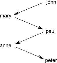
The situation is very different in the predicate logic / relational setting.  For example, look at this graph where an arrow $X \rightarrow Y$ indicates "$X$ loves $Y$":

That is a sad world.  This one is happier:

As a digression, sometimes I wonder if a multi-person cycle can exist in real life (eg, $John \rightarrow Mary \rightarrow Paul \rightarrow Anne \rightarrow John$), interpreting the relation as purely sexual attraction.  Such an example would be interesting to know, but I guess it's unlikely to occur.  </digression>

So the problem of relational learning is that data points cannot be represented in space with fixed labels.  For example we cannot label people with + and -, where "+ loves -", because different persons are loved by different ones.  At least, the naive way of representing individuals as points in space does not work.

My "matrix trick" may be able to map propositions to a high-dimensional vector space, but my assumption that concepts are matrices (that are also rotations in space) may be unjustified.  I need to find a set of criteria for matrices to represent concepts faithfully.  This direction is still hopeful.

How to make logic inference fast?

DPLL

The current fastest propositional SAT solvers are variants of DPLL (Davis, Putnam, Logemann, Loveland).  Davis and Putnam's 1958-60 algorithm was a very old one (but not the earliest, which dates back to Claude Shannon's 1940 master's thesis).

Resolution + unification

Robinson then invented resolution in 1963-65, taking ideas from Davis-Putnam and elsewhere.  At that time first-order predicate logic was seen as the central focus of research, but not propositional SAT.  Resolution works together with unification (also formulated by Robinson, but already in Herbrand's work) which enables it to handle first-order logic.

Resolution + unification provers (such as Vampire) are currently the fastest algorithm for theorem proving in first-order logic.  I find this interesting because resolution can also be applied to propositional SAT, but it is not the fastest, which goes to DPLL.  It seems that unification is the obstacle that makes first-order (or higher) logic more difficult to solve.

What is SAT?

For example, you have a proposition $P = (a \vee \neg b) \wedge (\neg a \vee c \vee d) \wedge (b \vee d)$ which is in CNF (conjunctive normal form) with 4 variables and 3 clauses.  A truth assignment is a map from the set of variables to {$\top, \bot$}.  The satisfiability problem is to find any assignment such that $P$ evaluates to $\top$, or report failure.

Due to the extreme simplicity of the structure of SAT, it has found connections to many other areas, such as integer programming, matrix algebra, and the Ising model of spin-glasses in physics, to name just a few.

The DPLL algorithm is a top-down search that selects a variable $x$ and recursively search for satisfaction of $P$ with $x$ assigned to $\top$ and $\bot$ respectively.  Such a step is called a branching decision.  The recursion gradually builds up the partial assignment until it is complete.  Various heuristics are employed to select variables, cache intermediate results, etc.

Edit:  DPLL searches in the space of assignments (or "interpretations", or "models").  Whereas [propositional] resolution searches in the space of resolution proofs.  I have explained resolution many times elsewhere, so I'll skip it here.  Basically a resolution proof consists of steps of this form:
           $$ \frac{P \vee Q, \quad \neg P \vee R} {Q \vee R} $$
As you can see, it is qualitatively different from DPLL's search.

How is first-order logic different?

It seems that unification is the obstacle that prevents propositional techniques from applying to first-order logic.

So what is the essence of unification?  For example, if I know
      "all girls like to dress pretty" and
      "Jane is a girl"
I can conclude that
      "Jane likes to dress pretty".
This very simple inference already contains an implicit unification step.  Whenever we have a logic statement that is general, and we want to apply it to yield a more specific conclusion, unification is the step that matches the specific statement to the general one.  Thus, it is unavoidable in any logic that has generalizations.  Propositional logic does not allow quantifications (no $\forall$ and $\exists$), and therefore is not compressive.  The compressive power of first-order logic (or above) comes from quantification and thus unification.

Transform logic inference to an algebraic problem?

I have found a nice algebraic form of logic that has the expressive power of higher-order logic and yet is even simpler than first-order logic in syntax.  My hope is to transform the problem of logic inference to an algebraic problem that can be solved efficiently.  So the first step is to recast logic inference as algebra.  Category theory may help in this.

Unification in category theory

In category theory, unification can be construed as co-equalizer (see Rydeheard and Burstall's book Computational Category Theory).  Let T be the set of terms in our logic.  A substitution $\theta$ is said to unify 2 terms $(s,t)$  if  $\theta s = \theta t$.  If we define 2 functions $f, g$ that points from 1 to T, so that $f(1) = s$ and $g(1) = t$, then the most general unifier (mgu) is exactly the co-equalizer of $f$ and $g$ in the category T.

The book also describes how to model equational logic in categories, but the problem is that the formulas in an AGI are mainly simple propositions that are not equational.  How can deduction with such propositions be recast as solving algebraic equations....?