
Getting the word lists
From this Wikipedia page, I got the lists of 100, 200, and 1000 basic English words.How to access WordNet from Python
Python is particularly good for accessing WordNet, thanks to this book and the NLTK library written by the authors.After installing NLTK (and the WordNet corpus), in Python, you can just:
>>> from nltk.corpus import wordnet as wn
>>> wn.synsets("cats")
and WordNet will return a bunch of "synonym sets" of the word cat. In this case they are:
[Synset('cat.n.01'), Synset('guy.n.01'), Synset('cat.n.03'), Synset('kat.n.01'), Synset("cat-o'-nine-tails.n.01"), Synset('caterpillar.n.02'), Synset('big_cat.n.01'), Synset('computerized_tomography.n.01'), Synset('cat.v.01'), Synset('vomit.v.01')]
Synsets are the basic unit of meanings in WordNet.
To get the similarity distance between 2 synsets, do:
synset1.path_similarity(synset2)
There are a bunch of XYZ_similarity measures, but their quality appears similar to each other. I did not try them all, as I found that the overall quality of WordNet as an ontology is problematic.
For more details, read the book's section on WordNet.
Basics of clustering
Suppose you have 1000 items, and you know the distances (ie similarity measures) between every pair of items. Then the clustering algorithm will be able to calculate the clusters for you. This is all you need as a user of clustering. The algorithm is also pretty simple (there are a number of variants), which you can find in machine learning textbooks. The idea is something like iterating through the set of items, and gradually creating and adding items to clusters.
The input is in the form of a similarity matrix, for example (I made this up, which is different from WordNet's):
The entries above the diagonal are not needed, because they're just the mirror image of the lower ones. This is called the lower triangular matrix. Sometimes the clustering library wants the upper one, then you need to do the matrix transpose, which is just exchanging the i, j indexes.

Sometimes the library function requires you to flatten the diagonal matrix into a linear array. Doing it row by row to the lower triangle, we'll get: [1.0, 0.6. 1.0, 0.5, 0.7, 1.0, 0.3, 0.3, 0.1, 0.1]. The mathematical formula for this is:
cell $(i,j)$ in matrix $ \mapsto $ element $j + i(i-1)/2$ in array
and the whole array is of size $n(n-1)/2$. Working out this formula may help you debug things if needs be. One common mistake is confusing lower and upper.
Another glitch is that the library may require dissimilarity instead of similarity values. So I have to do $(1.0 - x)$.
I find it helpful to generate a CSV (comma separated values) file and use OpenOffice Calc to inspect it, eg:

Where I wrote some BASIC scripts to highlight the diagonal and special values such as 1.0 and words with all entries empty. For example, I just need to "record macro", color a cell red, move the cell cursor 1 step down diagonally, and then add a For-Next loop around the generated BASIC code.
For PyCluster my incantation is:
from Pycluster import *
| cat | dog | man | worm | |
| cat | 1.0 | |||
| dog | 0.6 | 1.0 | ||
| man | 0.5 | 0.7 | 1.0 | |
| worm | 0.3 | 0.3 | 0.1 | 1.0 |
The entries above the diagonal are not needed, because they're just the mirror image of the lower ones. This is called the lower triangular matrix. Sometimes the clustering library wants the upper one, then you need to do the matrix transpose, which is just exchanging the i, j indexes.
This is a helpful illustration of transpose:
Sometimes the library function requires you to flatten the diagonal matrix into a linear array. Doing it row by row to the lower triangle, we'll get: [1.0, 0.6. 1.0, 0.5, 0.7, 1.0, 0.3, 0.3, 0.1, 0.1]. The mathematical formula for this is:
cell $(i,j)$ in matrix $ \mapsto $ element $j + i(i-1)/2$ in array
and the whole array is of size $n(n-1)/2$. Working out this formula may help you debug things if needs be. One common mistake is confusing lower and upper.
Another glitch is that the library may require dissimilarity instead of similarity values. So I have to do $(1.0 - x)$.
Looking at the data in a spreadsheet
Where I wrote some BASIC scripts to highlight the diagonal and special values such as 1.0 and words with all entries empty. For example, I just need to "record macro", color a cell red, move the cell cursor 1 step down diagonally, and then add a For-Next loop around the generated BASIC code.
Calling the clustering library
I tried 2 libraries:- PyCluster for Python
- FastCluster for R or Python
For PyCluster my incantation is:
from Pycluster import *
tree = treecluster(data=None, mask=None, weight=None, transpose=0, method='a', dist='e', distancematrix=triangle)
For R, I need to use a special function "as.dist()" to convert the lower triangle into a distance matrix before calling:
hc <- fastcluster::hclust(dis, method="single")
All my code is available here:
By the way, the code and the directory are unpolished. This is not my serious project. I just decide to share the raw stuff :)
Visualization
The output of R can be visualized simply by calling the dendrogram plot:
den <- as.dendrogram(hc)
plot(den, ylim=c(1,n), xlim=c(0,1), horiz=TRUE, dLeaf=-0.03)
The problem with R is that it's not easy to manipulate the visual looks (I couldn't find the relevant documentation online, but the book "R Graphics" may have what I need).
This is the dendrogram made by R (without appropriate labels):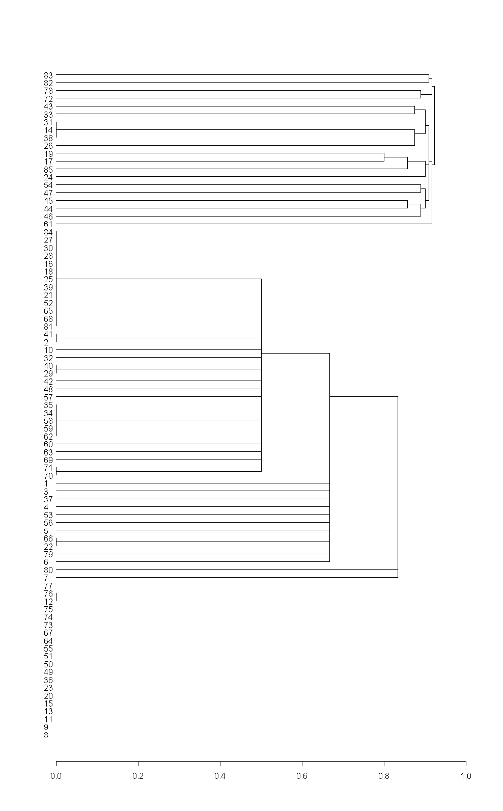
With Python I have more flexibility, by exporting to an external graph visualizer. I tried:
This is the dendrogram made by R (without appropriate labels):
With Python I have more flexibility, by exporting to an external graph visualizer. I tried:
- yEd
- GraphViz (Gvedit)
- Gephi
- Ubigraph
yEd is my favorite (whose output you see), and it accepts GraphML files as input. I just saved a test file of the visual style I want, then emitted my data in GraphML format, from Python.
GraphViz Gvedit is similar, but accepts .DOT files. .DOT is even simpler than GraphML. For example, this is a .DOT directed graph:
digraph G {
man -> woman
dog -> cat
}
But GraphViz's layout function is not so intuitive to use (ie, it requires reading about and typing parameters, whereas yEd provides a GUI. Of course a lazy person as me eschews that).
Gephi looks quite sophisticated, but unfortunately it is unstable on my Windows XP, and I also tried it in Linux virtual box, also failed. Perhaps the reason is it requires OpenGL which must be installed from your video card's manufacturer, and my version was outdated and I couldn't fix it. A nuisance. If you think your OpenGL version is good, you may try it.
Ubigraph lets you visualize graphs dynamically. It runs a server which can be easily accessed via remote RPC protocol. So I can see my graph's nodes spring out in real time, click on nodes and program its behavior, etc. But, it gets slow after a while as the graph grows big. Also, the Ubigraph project is now out of maintenance. Some functions are still imperfect...
Last but not least
Some people have noticed the "loners left out" double entendre in my last post, but it was originally unintended. Afterwards I realized I've hit on something very interesting :)
I've started to get involved in social entrepreneurship, and came across the idea of the importance of social inclusion. Milton's phrase "They also serve who only stand and wait" was in the back of my mind when I wrote that.


