Latex Maths

Friday, October 26, 2012

Playing with WordNet (the code)

This is how I did it:

Getting the word lists

From this Wikipedia page, I got the lists of 100, 200, and 1000 basic English words.

How to access WordNet from Python

Python is particularly good for accessing WordNet, thanks to this book and the NLTK library written by the authors.

After installing NLTK (and the WordNet corpus), in Python, you can just:

>>> from nltk.corpus import wordnet as wn
>>> wn.synsets("cats")

and WordNet will return a bunch of "synonym sets" of the word cat.  In this case they are:

[Synset('cat.n.01'), Synset('guy.n.01'), Synset('cat.n.03'), Synset('kat.n.01'), Synset("cat-o'-nine-tails.n.01"), Synset('caterpillar.n.02'), Synset('big_cat.n.01'), Synset('computerized_tomography.n.01'), Synset('cat.v.01'), Synset('vomit.v.01')]

Synsets are the basic unit of meanings in WordNet.

To get the similarity distance between 2 synsets, do:

    synset1.path_similarity(synset2)
There are a bunch of XYZ_similarity measures, but their quality appears similar to each other.  I did not try them all, as I found that the overall quality of WordNet as an ontology is problematic.

For more details, read the book's section on WordNet.

Basics of clustering

Suppose you have 1000 items, and you know the distances (ie similarity measures) between every pair of items.  Then the clustering algorithm will be able to calculate the clusters for you.  This is all you need as a user of clustering.  The algorithm is also pretty simple (there are a number of variants), which you can find in machine learning textbooks.  The idea is something like iterating through the set of items, and gradually creating and adding items to clusters.

The input is in the form of a similarity matrix, for example (I made this up, which is different from WordNet's):

catdogmanworm
cat1.0
dog0.61.0
man0.50.71.0
worm0.30.30.11.0

The entries above the diagonal are not needed, because they're just the mirror image of the lower ones.  This is called the lower triangular matrix.  Sometimes the clustering library wants the upper one, then you need to do the matrix transpose, which is just exchanging the i, j indexes.

This is a helpful illustration of transpose:

Sometimes the library function requires you to flatten the diagonal matrix into a linear array.  Doing it row by row to the lower triangle, we'll get:  [1.0, 0.6. 1.0, 0.5, 0.7, 1.0, 0.3, 0.3, 0.1, 0.1].  The mathematical formula for this is:
    cell $(i,j)$ in matrix $ \mapsto $ element $j + i(i-1)/2$ in array
and the whole array is of size $n(n-1)/2$.  Working out this formula may help you debug things if needs be.  One common mistake is confusing lower and upper.

Another glitch is that the library may require dissimilarity instead of similarity values.  So I have to do $(1.0 - x)$.

Looking at the data in a spreadsheet


I find it helpful to generate a CSV (comma separated values) file and use OpenOffice Calc to inspect it, eg:


Where I wrote some BASIC scripts to highlight the diagonal and special values such as 1.0 and words with all entries empty.  For example, I just need to "record macro", color a cell red, move the cell cursor 1 step down diagonally, and then add a For-Next loop around the generated BASIC code.

Calling the clustering library

I tried 2 libraries:


For PyCluster my incantation is:
from Pycluster import *

tree = treecluster(data=None, mask=None, weight=None, transpose=0, method='a', dist='e', distancematrix=triangle)

For R, I need to use a special function "as.dist()" to convert the lower triangle into a distance matrix before calling:
hc <- fastcluster::hclust(dis, method="single")

All my code is available here:
By the way, the code and the directory are unpolished.  This is not my serious project.  I just decide to share the raw stuff :)

Visualization

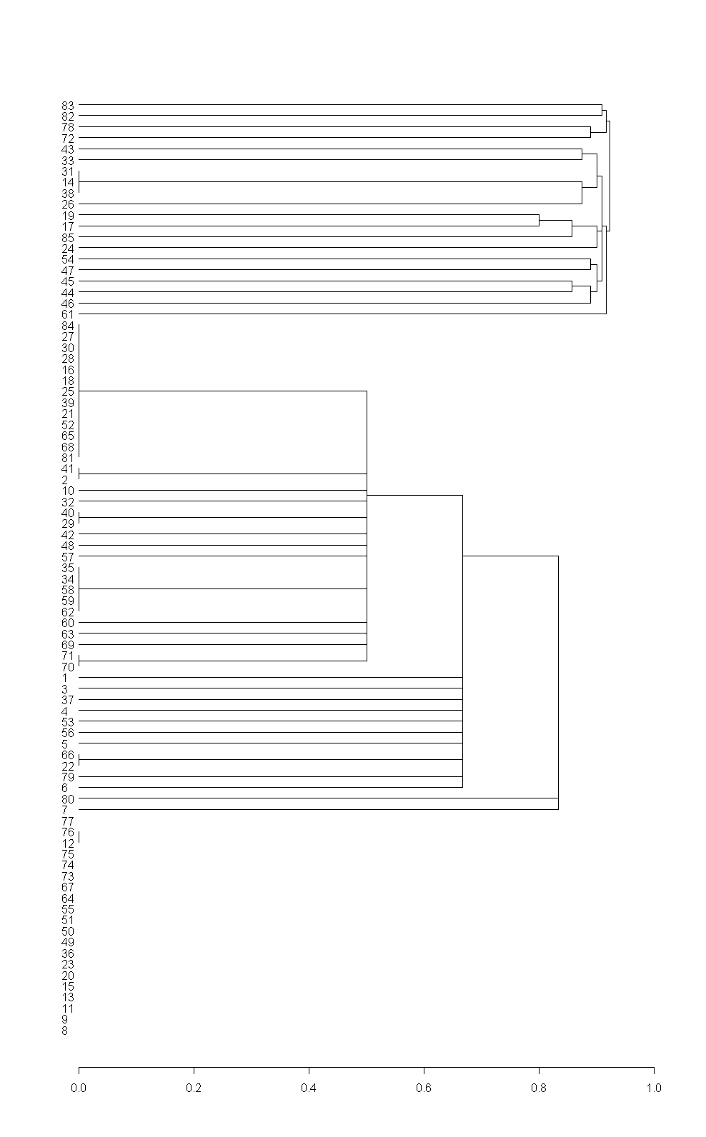
The output of R can be visualized simply by calling the dendrogram plot:
den <- as.dendrogram(hc)
plot(den, ylim=c(1,n), xlim=c(0,1), horiz=TRUE, dLeaf=-0.03)

The problem with R is that it's not easy to manipulate the visual looks (I couldn't find the relevant documentation online, but the book "R Graphics" may have what I need).

This is the dendrogram made by R (without appropriate labels):
With Python I have more flexibility, by exporting to an external graph visualizer.  I tried:
  • yEd
  • GraphViz (Gvedit)
  • Gephi
  • Ubigraph
yEd is my favorite (whose output you see), and it accepts GraphML files as input.  I just saved a test file of the visual style I want, then emitted my data in GraphML format, from Python.

GraphViz Gvedit is similar, but accepts .DOT files.  .DOT is even simpler than GraphML.  For example, this is a .DOT directed graph:

   digraph G {
       man -> woman
       dog -> cat
   }

But GraphViz's layout function is not so intuitive to use (ie, it requires reading about and typing parameters, whereas yEd provides a GUI.  Of course a lazy person as me eschews that).

Gephi looks quite sophisticated, but unfortunately it is unstable on my Windows XP, and I also tried it in Linux virtual box, also failed.  Perhaps the reason is it requires OpenGL which must be installed from your video card's manufacturer, and my version was outdated and I couldn't fix it.  A nuisance.  If you think your OpenGL version is good, you may try it.

Ubigraph lets you visualize graphs dynamically.  It runs a server which can be easily accessed via remote RPC protocol.  So I can see my graph's nodes spring out in real time, click on nodes and program its behavior, etc.  But, it gets slow after a while as the graph grows big.  Also, the Ubigraph project is now out of maintenance.  Some functions are still imperfect...

Last but not least

Some people have noticed the "loners left out" double entendre in my last post, but it was originally unintended.  Afterwards I realized I've hit on something very interesting :)

I've started to get involved in social entrepreneurship, and came across the idea of the importance of social inclusion.  Milton's phrase "They also serve who only stand and wait" was in the back of my mind when I wrote that.

Saturday, October 20, 2012

Playing with WordNet (first impressions)

What I want is to build an ontology for use with common-sense inference.  An ontology induces a distance measure amongst words (or concepts), which can be used to distribute the concepts inside a high-dimensional sphere, with the concept of "everything" at the center.  This will be useful for my "matrix trick" (which I have explained in some slides, but I'll write about it later in this blog).

So, what I had in my mind was an ontology that looked like this (I just made this up):


But I quickly found out that the reality of ontologies is very different from what I expected!

The first problem is that WordNet has too many words, but I want to load an upper ontology into main memory and still be able to do inference search.  So my idea is to mine the ontology on demand.  For example, if I need an upper ontology of 1000 basic English words, then I can just construct the ontology by looking up the relevant relations in WordNet.

The idea seemed nice, but I found out that WordNet has too many hypernyms (= super-classes) for nouns and almost no hypernyms for adverbs.  For example, look at this visualization of the hypernyms of "cat" and "dog":

We have some surprises such as "a dog is a kind of unpleasant woman".

Also, some meanings are not what we expect, for example, for "cat" to mean a whip, or for "dog" to mean a mechanical device.  Because there is no fuzziness or probabilities, it is hard to distinguish between common and uncommon usage.

The red lines are links that connect "cat" to "dog".  There is the obvious connection via "carnivore" but there are also 2 other connections based on slang usage.

This is just the visualization of 2 iterations of hypernyms.  If we continue like this, the number of hypernyms will grow very large before they start to converge (because everything will ultimately end up as "entity").

This is a visualization of 1 step of hypernyms (blue) for 100 basic words (red):

Notice that at the bottom there are some loners left out of the game because they have no hypernyms (mostly adverbs).  Nevertheless, they are important words and should be included in a good ontology of concepts.

This is the visualization of 2 steps of hypernyms (blue) for 100 basic words (red):

The iteration will terminate ~10 steps for most branches, leaving us with 1000's of nodes and 100K's of linkages.  It is a non-trivial algorithmic problem to prune the graph.  Also disappointing is the fact that this graph will have many more intermediate nodes than the basic English words we started with -- something that I didn't expect.

At this point I gave up and started to try another method:  WordNet provides some similarity measures (such as "path_similarity") between words.  Maybe I can use these distances to cluster the words flatly?

This is a visualization of the similarities between 100 words:

As you can see, again, some adverbs or special words are left out at the bottom.

Also, there is no strong link between "left" and "right" (the strength is only 0.333, relatively low).  This is where I think WordNet's way of defining similarity in [0,1] is wrong.  Similarity should be measured in [-1,1] so that opposite concepts can be measured properly.

My conclusion so far:  "In artificial intelligence, avoid hand-crafting low-level data;  It's usually better to machine-learn!"

Looking forward: we may have to set up Genifer like a baby to learn a small set of vocabularies.  Or, we can use a flawed ontology but somehow supplement it to correct the deficiencies...  (Perhaps WordNet wasn't designed for using adverbs in a way similar to nouns.)

Sunday, February 12, 2012

unification = the calculus of concepts

Today I just had an insight:

Haskell Curry proposed combinatory logic as a logica universalis, but it ran into inconsistency problems.  (I'm trying to use fuzzy-probabilistic truth values to get around that problem, but that's a different topic.)

So, in 1963 JA Robinson discovered resolution, which is really unification + propositional resolution.  Unification decides if 2 terms can be made equationally identical.  Propositional resolution deals with the "calculus of thinking" at the proposition level.

Combinatory logic provides a free way to compose terms via "application".  I regard terms as concepts.  For example:
   "tall handsome guy"
is the combination of the concepts
   tall ∙ (handsome ∙ guy).

Now, a few examples:
"tall handsome guy" is equivalent to "handsome tall guy";
"very tall guy" implies "tall guy";  but
"very tall guy" does not equal "tall very guy";

Thus the unification theory is modulo some special rules akin to commutativity, associativity, etc, and certain reduction rules.  In other words, unification modulo a theory = "the calculus of concepts".

So we have a neat decomposition:
    calculus of thoughts = calculus of concepts
                                    + calculus of propositions

Video: Genifer in 4 minutes

This was made 2 months ago.  Just posting it here so people can find it from our blog:

Saturday, July 23, 2011

Distributive agents, illustrated

The following illustrates how deduction (backward-chaining) is performed.  Forward-chaining works very similarly.  I have left out how the agents find others to answer queries -- this is the routing strategy which is an optimization problem.

Agent2 performs only one step, namely, the resolution of:
  • P\/Q (the query Agent2 is being asked)
    with
  • ~P\/Q (the rule that Agent2 has in its KB)


This is another illustration, using a common-sense example:


By the way, the implication statement "A implies B":
     nice(X) ← sandals(X)
is classically equivalent to "not A or B":
     ~sandals(X) \/ nice(X)
and therefore it can be resolved with
    nice(matt)
by the substitution { X / matt }, yielding the resolvent:
    sandals(matt).
This is why the resolution step works.

Thursday, June 16, 2011

Distributive architecture for inference engine (deduction)

Eureka!! This new architecture is much simpler:


Each agent responds to queries and spits out solutions. For example, if you believe that "professors who wear sandals are nice to students" then you listen to queries about "who is nice to students". When there is a hit, you either:
  1. return an answer, if you know as a fact that XYZ is nice to students. 
  2. return a sub-goal, in this case, "does XYZ wear sandals?" and wait for others to answer. 
In case #2, if you got an answer "Professor Matt Mahoney wears sandals", say with TV = 0.9, then you decide how to calculate the TV of the conclusion given that TV of premise = 0.9. The only calculation you need to perform is for the rule that you own. Then you return the answer to the asker.

This architecture is so wonderful because there is no need to construct the proof tree anymore. The proof tree seems to have disappeared but it is really implicitly constructed within the network of agents!

Thanks to Matt Mahoney for proposing the CMR (competitive message routing) architecture.

For reference, this is an older design that reveals my thinking:  (This can be seen as a single agent, building the proof tree internally while trying to answer 1 query.  In the new architecture each agent is responsible for applying only one rule at a time).

Saturday, May 28, 2011

Self-programming architecture

This is not a new idea -- Ben and Jared in Opencog has mentioned it before (in the context of MOSES):


Abram seems to have an idea where the GP is replaced by RL (reinforcement learning).

Yesterday I was analyzing the GP + IE idea in more details:
  1. Let the GP side and the IE side gradually evolve in cycles, starting with $GP_1 + IE_1$.
  2. The key question is whether the cyclic route is faster than hand-coding IE.  Initially, it would involve more work because the GP side needs to be custom-made (we cannot use off-the-shelf GP software).  It may pay off only if $GP_1 + IE_1$ increases programming productivity significantly.
  3. A very weak $IE_1$ cannot increase programming productivity because GP + weak IE is still too slow to be usable.  For example, one idea is to have IE suggest a number of primitive functions when given a goal, so GP can include those primitives in the genes for that population.  But, even with current state-of-the-art GP, this cannot efficiently solve > 1 line programs, even if primitives are suggested.
  4. $IE_*$ (the ideal form of IE) will be able to deduce the program when given the desired goal: $$ G:goal \mapsto \{ P:program | \quad P \vdash G \}. $$ Whereas the above $IE_1$ is too weak (suggesting primitives similar to the goal): $$ G:goal \mapsto \{ x | \quad x \approx G \}. $$ Perhaps we need to find something in between weak $IE_1$ and $IE_*$.
  5. In other words, we simply have to hand-code $IE_1$ to reach a certain level of functionality before putting it to use with GP.  That basic level seems to include:
    • Ability to express simple plans (so that human teachers can supply basic programming knowledge as decomposition of tasks into sub-tasks)
    • Ability to express similarity and to perform simple associative recall.
    Interestingly, the ability to perform deduction seems not required for $IE_1$, nor the ability to calculate truth values.
The new insight may change our priorities during implementation...

Wednesday, September 8, 2010

Genifer: Facts and Rules Visualization

depth=3, 2D

depth=4, 3D


This interactive visualization is created by a GeniferGraph adapter class which exposes GeniferLisp's internal data to dANN.  dANN then uses the graph representation to dimensionally embed it in N-dimensional space.

Here is the sourcecode for the GeniferGraph class.  Notice that it uses recursive descent to add all LISP symbols to a finite depth.