什么是机器学习？ What is machine learning? (Chinese)

机器学习是 AI 最重要部分，但我上次用 Clojure 写 Genifer 的时候没有完成这部分，结果那 prototype 完全没有应用，是一大失误。

「学习」的本质

人脑很多时是通过「一般化 , generalization」来学习的。

例如，广东话俗语说：『有须就认老窦』(有胡子便认做父亲，用来取笑过份的一般而论)，但可能婴儿就是这样辨认亲人的。

又例如，小时候爷爷教我写中文的「一二三四五」，学到 3 的时候我便自作聪明地说：「我知道了，四字的写法是 4 划！」  虽然是错误的，但表示小孩子的思想方式。

又例如，有些人被女人骗过一次之后，便永远不信女人。

这些都是 generalization 的例子。

相反的方向叫 specialization (特殊化)，或 refinement (精细化)。

例如我们从「所有女人都说谎」修正到「有些女人是诚实的」，或者「那个骗我的女人其实也有诚实的一面。」

一般化 和 特殊化 就是逻辑学习的基本运作，没有别的内容了。

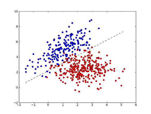
此外还有一种机器学习的範畴，是基於在空间中的点的模式识别：

例如我们已经知道有两类东西 (分别标作红色和蓝色)，而我们数量化地量度它们的某些特徵，然后在座标空间上点描出来，这时发现红点和蓝点的分布大致可以用一条线分割，於是以后我们只要量度那些特徵，就可以分辨哪些是红组或蓝组的东西，而不需要知道事先知道它们的颜色。

这种「空间中」的统计学习 (statistical learning)，其先决条件是知道一些数值上的量度，否则根本没有几何空间可言。  神经网络就是这种 "spatial learning" 的例子。

On the other hand，逻辑学习是不需要几何空间的，它只需要「符号」运作 (symbolic manipulations)。

以下我们专注逻辑学习；  如何统一逻辑学习和空间学习，我觉得是研究的重要课题。

Logic-based learning

例如说，我们观察到「很多读电脑的人都戴眼镜」，但我们是怎样跳到这个「归纳」的结论的？

在逻辑引擎中，已经有的 gound facts (事实资料) 是：
读电脑(小明)， 戴眼镜(小明)，
读电脑(小娟)， 戴眼镜(小娟)，
读电脑(小强)， 戴眼镜(小强)，
读电脑(美玲)， 戴眼镜(美玲)，
读音乐(小芬)，不 戴眼镜(小芬)，
男生(小明)，男生(小强)，
女生(小娟)，女生(美玲)，女生(小芬)，
. . . . . . . 等等。

我们欲求得到的 general rule 是：
读电脑(X) $\rightarrow$ 戴眼镜(X)

其实那算法就是在所有可能的 formula 里面搜寻。

换句话说，由最简单的 formula 开始，我们不断 generate 越来越复杂的 formulas，然后我们逐一试验这些 formulas，看看哪一条最能解释事实。

最简单的 formula 就是一条「空」的命题 (什么也没有，表示一切都是真的)。

然后我们逐步添加一些逻辑项 (terms)。

例如：
$\rightarrow$ 戴眼镜(X)
表示任何人都戴眼镜，但那和事实不符。

又例如：
女生(X) $\rightarrow$ 戴眼镜(X)
「所有女生都戴眼镜」，那也和事实不符。

最后我们试验：
读电脑(X) $\rightarrow$ 戴眼镜(X)
发现其机率很高 (或许有少数例外)，於是接受这一假设。

换句话说，这是在「假设空间，hypothesis space」中的搜寻。

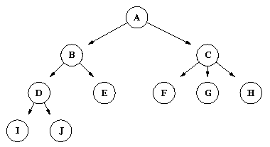
这些 search space (搜寻空间) 的结构，形状像「树」那样不断细分下去：


我们由最「一般」的命题 (什么都是真的) 开始搜寻，到越来越特殊的命题，例如「22 岁、五月生日、体重 70 公斤以上、读大学 4 年级、数学不合格、姓张的人 $\rightarrow$ 都戴眼镜」，这过程中必然会出现我们期待的 formula。  这叫 general-to-specific search。

但由於 假设空间里面 有非常多组合 (combinatorial) 的可能性，所以这种学习是很慢的。

似乎唯一的解决之道，就是把所有概念和法则都分类，例如「这是属於物理学的知识」、「这是关於我女朋友的知识」…… 等，而在搜寻时我们只关注那些最可能有关的集合，例如「买礼物给女友时 考虑 class A 的知识」、「物理学考试时 考虑 class B 的知识」 …… 等等。

虽然很难，但必须把这个算法写出来，否则 Genifer 便无望了！

PS:  我在 Genifer 网页里有更详细解释 inductive learning (PDF, in English)。

如何写一个逻辑引擎？How to write a logic engine? (Chinese)

现试用最简单的方法，介绍如何写一个逻辑引擎。

即使是现时最尖端的人工智能，例如 OpenCog，它的内部仍然是很简单的。

逻辑推理 (deduction) 只需要两个算法：

1. 命题推理
2. 配对法 (unification) 

这两个算法只需要数行程式就能表达 !

逻辑是什么？

逻辑可以分解为两部分:

1. 命题逻辑 (propositional logic)
2. 命题内部的结构

命题逻辑

命题逻辑的意思是：  我们只关心命题的真假，而不看命题内部的结构。  所以「小明爱小娟」和「北京昨天下雨」都是同一类句子，只要我们知道它们的真值 (truth value)。

命题之间的关系用箭頭表示，例如：

1. 吃了不洁食物 $\rightarrow$ 肚痛
2. 下大雨，没带雨伞 $\rightarrow$ 变落汤鸡

但命题不一定非黑即白，关系也会有不确定因素，所以最严格是要用 fuzzy probability (模糊 机率) 来描述。

推理的算法，原理很简单：

所有命题的关系构成一个 graph，例如下图：

有些 nodes 的真值我们知道，有些不知道； 我们将真值由已知的 nodes「传播」到未知的 nodes 去。 这传播有其法则，例如 机率 要用机率论的法则计算，你甚至可以自创，甚至可以用机器学习那些法则，而不需我们伤脑筋去设计！

所以，你只要懂得怎样在电脑建立和处理 graph 结构，第一个问题便解决了。

谓词逻辑

现在来看看句子内部的结构。

最经典的做法是用谓词逻辑 (predicate logic)，那是 Gottlob Frege 在 1879 年发明的。  罗素 (Bertrand Russell) 用它改写所有数学，使之发扬光大，然后 AI 之父 John McCarthy 把它应用在 AI 上，变成 classical AI。  但现在我们搞 strong AI 的人似乎都不太喜欢它，使用一些变奏，但基调一样。

谓词逻辑的做法就是将句子拆成 predicate 和 predicate 里面的 objects。
例如：
「小明爱小娟」 -->  爱(小明，小娟)
「北京下雨」-->  下雨(北京)
但对於较为复杂的句子结构例如「小明执迷不悟地爱着小娟」则视乎个别研究者的做法，没有统一的准则。  我们暂时不深究。

其实只要用某个方法把句子内部拆开就行，命题的推理方法完全没有变。

但句子拆开之后，我们可以在里面使用 variables (变量)，那是很有用的。

例如，我们可以构造：
爱(小明，X)
那变量 X 可以是 小娟、美玲、等。

於是现在我们需要另一个算法，叫 unification (配对)。

Unification

Unify 的作用是：  给定两个句子 A 和 B，它们内部可以很复杂，也可以有 variables，而我们试图找一些 substitutions (代入)，令那两句变成一样。

例如：
爱(X，Y)
和
爱(小强，美玲)
这两句命题，只要代入｛X = 小强，Y = 美玲｝，就可以变成同一句。

当然有些命题是无法 unify 的，例如：
爱(小明，小娟)
恨(小明，X)
那算法便会回覆 "fail"。

变量是很重要的发明，有了变量才可以表达 general rules (一般法则)，例如：
「女人都说谎」换成逻辑就是：
女人(X) $\rightarrow$ 说谎(X)

有些人被女人骗过一次之后，便永远不信女人；  所以人脑的思想也是透过 generalization (一般化) 来学习的。  那是机器学习的範围，容后再谈。

Unify 所做的其实是 pattern matching。
例如：
    戴眼镜(X) 或 爱(小明，Y)
是一些模式，可以套到：
    戴眼镜(美玲) 或 爱(小明，小娟)
这些实例上。

人工智能就是一个很大的资料库，里面有很多用模式写成的 general rules，经过配对而产生新的推论。  例如 小娟是女人，所以用上面那条 general rule，得出小娟说谎的结论。 

Cayley graphs of free groups and monoids

This is a Cayley graph:



Its nodes represent elements of the free group generated by {a, b}.  It goes out in 4 directions from the origin:  ${a, b, a^{-1}, b^{-1}}$.

This is an animated GIF of the same graph:

But it only recursively repeat in 3 directions, as $a \cdot a^{-1} = 1$ ("going backwards") is cancelled out.

The graph itself is of fractal dimension, but it is embedded on the 2D plane (of dimension 2), that is because the group is generated by 2 elements.

If we ignore the non-commutativity of the group, in other words $a \cdot b = b \cdot a$, then we don't have to shrink the edges, and the Cayley graph becomes a regular grid like this:

This can be regarded simply as the direct product of the generator groups {a} and {b}.  And it clearly shows why 2 dimensions are needed.

But interestingly, we can also plot the Cayley graph of a free group with 3 elements on the 2D plane.

My first attempt is to divide the full circle of $360^\circ$ into 6 points, with 3 points representing {a, b, c} and 3 others the inverses.  But unfortunately there is a "clash" between some elements:

So the solution is to shrink the edges not by 1/2 but by 1/3.  This is the result:

This trick can work for any number of generators, by just cutting 2n divisions of the full circle.  For example this is case n=4:

Case n=10:

Free monoids

What if we ignore the inverse elements, so we get free monoids?  We can have 4 elements {a, b, c, d} and the graph is as follows:

It is clear that the nodes are "space-filling" as every point in the square can be expressed as a binary fraction.

Thus every point uniquely identifies a word in the free monoid generated by 4 elements.  Beware that some edges are overlapping in this graph.

The case of n=3 monoid is a bit interesting, as it turns out to be the Sierpinsky triangle!

When n gets big, the monoid graphs looks exactly the same as the group graphs for n/2.  For example, this is monoid, n=20:

And this is monoid, n=100:

Code

The code is very short, written in HTML5 Canvas and Javascript.  You can download the .zip here.

Why the interest?

I am interested in this because the free groups / monoids can represent logical formulas (when the logic is in algebraic form).  If we add a "gray scale" or "colors" to the nodes, that gives them extra dimensions that can be regarded as truth values.  Thus, an entire knowledge base can be represented by such a continuously-colored graph.

In other words, we have a geometric representation of knowledge elements that can be multiplied and added together.  Multiplication is the monoid action, whereas addition is the scalar addition of truth (color) values.

I will write about this last idea in more details.... later :)

P = NP, my first stab at the problem

[ This idea is inspired by Karmarkar's polynomial-time interior point method for linear programming. But it turned out to be a dead end, at least from my current perspective.  Anyway, I leave the record here for future's sake and it might illuminate other people.  ]

In mathematics, there is a long tradition of using "smooth" things to calculate "discrete, combinatorial" things. A famous early example is Euler's use of Newton/Leibniz's integral to approximate infinite series of the form $ \sum^n_{i=1} f(i) $, also known as Euler-Maclaurin summation [cf the book "Mathematical Masterpieces", Knoebel et al 2007]. A more recent example is Alexander Grothendieck's invention of schemes that builds a bridge between the (smooth) algebraic geometry and (discrete) Diophantine geometry.

So my hunch is to "move the SAT problem to a smooth setting and then apply smooth techniques". In fact, that was exactly what happened for the linear programming problem -- the simplex algorithm is discrete in the sense that it traverses the vertex points on the boundary of the feasible solution space, such a traversal tends to be exponential because the number of vertices grows exponentially as the number of equations. Whereas, the "interior point" methods avoid the boundary and vertices and instead manipulate "ellipsoids" that bound the feasible space.

Using an analogy, imagine a hotel with an exponential number of rooms, where some of the rooms contain the prize, but we have only a polynomial amount of time to check the rooms. On the surface it seems impossible; that is why P=NP is hard. But it is only the size of the ambient space that is exponential; the targets are finitely generated from a description of length N (= the input size); so there is hope.

Now add to the mix the inspiration from "interior point" methods: our algorithm should avoid testing the hotel rooms -- because as soon as we test the first room we may get trapped into testing an exponential number of rooms, just as in linear programming we have to avoid "touching" the boundary. Perhaps we should iterate through the input constraints, updating a certain "data structure" (which could be any mathematical structure in a broad sense), and such a structure would asymptotically approach the feasible solution(s).

The final shape of this data structure cannot contain the entire solution set, since it has an exponential number of vertices, and there isn't enough time to update that many vertices before the answer should be out. It cannot even contain a subset of those vertices, because then some of the vertices have to be eliminated in the process, thus making our function discontinuous. (Topologically, continuous means that the pre-image of every open set remains open).

Our function cannot output [0,1] because the answer may jump between 0 and 1, again discontinuous.

Notice that SAT is equivalent to deciding whether a set of polynomials have solutions in the reals ("existential theory of the reals"). Currently the best algorithm for this is singly exponential [cf: "Algorithms in real algebraic geometry", Basu et al 2006, ch.13].

But our function cannot output the volume of the set of real solutions, as the volume depends on the entirety of the boundary, which we want to avoid. The Oleinik-Petrovsky-Thom-Milnor theorem [cf Basu et al 2006, p.4] set a bound on the sum of Betti numbers of an algebraic set, which is polynomial in the degree and exponential in the number of variables. The first Betti number is the number of connected components of the set. This seems to confirm my intuition that the boundary is of "exponential" complexity and thus should be avoided.

After eliminating these options, there may still be a viable path which is to find the "minimal" real solution in the algebraic set.  That means we take only the real component of z and require that its Euclidean norm, $||Re z||_2$, be smallest.  A slight glitch is that the real part of a complex number is given by $Re z = z + z^*$ where $z^*$ denotes complex conjugation, which cannot be expressed in a polynomial formula.

But I realized that a fatal problem of this approach is that we still have not avoided testing an exponential number of points.  This can be illustrated by this picture:

The regions are defined by a set of $k$ polynomials of maximum degree $m$, in $n$ variables.  We need to find the common intersections (if any exists) of all $k$ polynomials.  Figuratively speaking (as this diagram is not realistic), the potential number of intersections is related to the number of "peaks", ie the degree of the polynomials.

If we must test each "peak" against each other, for all $k$ polynomials, the maximal number of tests would be $m^k = O(m^n)$, ie, exponential in the number of variables.

To put it succinctly, the problem is:  When we test a peak at a certain location, our effort spent at that location does not contribute to testing the peaks at other locations, and we have an exponential number of peak-to-peak combinations to be tested.

This is the general feeling one has when tackling an NP-hard problem.

So, the critical insight that may ultimately solve NP is that we should not waste time testing local cases, but we should exploit the fact that the localities are somehow correlated to each other.

It is well known that 2-SAT is in P and 3-SAT is NP-complete.  In other words, when the degree of the polynomials gets to 3, we get NP-hardness.  Any degree-higher-than-3 problems can be reduced to degree-3 instances, so we only need to consider cubic surfaces.  That would be my next goal.... :)

P = NP can be proven?

I have a hunch that P=NP can actually be proven.

It is known that in this chain of inclusions:
$$ P \subseteq NP \subseteq PSPACE \subseteq EXPTIME $$ at least one inclusion is proper (ie, equality does not hold), by the "Time Hierarchy theorem". Other than that, none of the inclusions have been proven to be proper so far. Note that this theorem is proved via diagonalization, ie, Cantor's theorem that the cardinality of a power set must be bigger than the cardinality of the set itself. In other words, the proof is based on cardinality. But (with my limited knowledge and saying this vaguely) I have not known of similar cardinality proofs that are "smaller" than Cantor's. Does it mean that there is only 1 inequality within that chain?

What is Montague grammar?

Montague grammar

Richard Montague developed his theory of grammar from 1950-1970s.  What is special about Montague grammar is that, whereas Chomsky's transformational grammar provides a formal account for the syntax of natural language, Montague grammar has both formal syntax and semantics.

Basically, Montague uses categorial grammar to describe the syntax of a natural language.  Then he establishes formal translation rules that maps natural-language sentences to logical formulas in intensional logic.  Such formulas have well-defined semantics based on possible worlds.

Let's turn to the semantics first, since it is the most interesting and relevant to AGI...

Intensional logic (內涵邏輯)

Intensional logic originated as an attempt to resolve paradoxes due to confusing references with senses (指涉 和 涵義), or extensions with intensions (外延 和 內涵).  Its idea has been studied by Frege (1892), Lewis (1914), Tarski (1933), Carnap (1947), Kripke (1963), Montague (1970).

To say that:
       The Empire State Building is the tallest building in New York
is not the same as saying:
       The tallest building in New York is the tallest building in New York
even though we have substituted equal by equal.  How come?

The problem is that "the tallest building in New York" is a symbol that has a reference (or extension) which is the object it refers to, and a sense (or intension) which is more subtle and depends on the context under which it is interpreted.

In different possible worlds (such as different time periods), "the tallest building in New York" can refer to different objects.  While the extension of a symbol can be taken as the set of individuals it refers to, the intension of the symbol cannot be such a set, but has to be the function that maps from possible worlds to individuals in the worlds.  As shown in the diagram:

In other words, the function associates to each possible world an individual in that world which the symbol refers to.  That is:

$ f: I \rightarrow U $

$ f: i \mapsto u $

where $I$ is the set of possible worlds (or interpretations), and $U$ is the set of individuals that figure in any of the worlds.

The intensional logic (IL) as described by Montague is a meta-language based on $\lambda$-calculus, that allows to define various modal operators, so that it can subsume modal logic, temporal logic, deontic logic, and epistemic logic, etc.

Compound nouns

I discovered that intension functions may also help us define the semantics of compound nouns, such as:

cyber sex	sex that happens on the internet
glass slippers	slippers made of glass
couch potato	person who stays in the couch all the time

Some compound nouns are easy to interpret as they are simply the conjunction of their constituent atomic concepts.  For example, a "girl scout" is both a "girl" and a "scout".  However, a "girl school" is not a "girl", but is for girls.  The meaning of such atypical compound nouns seem to require abductive interpretation (溯因解釋).  Abduction means to search for explanations for what is known, which is the reverse of deduction which searches from what is known to new conclusions.

Now with the insight from intensional logic, perhaps we can interpret compound nouns like this:

So each modifier is a function that maps from possible worlds to individuals.

The advantage of such a treatment is that concept composition in general can be uniformly represented by intensional logic.

What is a function?

When we say "there exists a function...", it can be deceptive as the function can be any arbitrary mapping -- for example, it can include a bizarre map that maps an individual to Confucius in world$_1$, to the number 7 in world$_2$, to the Empire State Building in world$_3$, etc.  What we need is to operationalize the concept of functions.

In the logic-based paradigm, a function is implemented as a set of logic formulas that determine the elements of a predicate.  For example, the Prolog program:
    ancestor(X,Y) :- father(X,Y)
    ancestor(X,Y) :- ancestor(X,Z), father(Z,Y)
    etc...
determines the elements of the "ancestor" relation.

So we have found an operational implementation for functions, and as logic programs are Turing universal, they are also the broadest class of functions we can define.  One question is whether we can simplify the logical form, while keeping its Turing universality.

Possible world semantics

Possible world semantics were developed by Carnap and Kripke, among others, but Leibniz was the first "logician" to use the term "possible world".

The relevance to intensional logic is that each intensional individual is a function from the set of possible worlds (W) to the set of possible individuals (D):
    $ f : W \rightarrow D $.
In other words, the set of all intensional individuals is $D^W$.

Possible world semantics is a way to model modal logics (模態邏輯).  Modal logic is distinguished by the use of the modal operators $\Box$ "necessarily" and $\diamond$ "possibly".  To model a logic means to establish a correspondence between propositions (命題) in the logic and an underlying algebraic structure called interpretations, such that the truth of propositions in the logic can be determined (or evaluated) by looking into that algebraic structure.  In the case of modal logic, its model can be given by Kripke structures, or possible worlds.

What is a Kripke structure?  It is a tuple $\left< W, R, V \right>$ of possible worlds $W$, a binary accessibility relation $R$ between worlds, and a valuation map $V$ assigning {true, false} to each proposition $p$ in possible world $w$.

Modal truths are defined by this interpretation rule:
     $ \Box \phi \Leftrightarrow \forall w \in W. \phi $
which means that $\phi$ is necessarily true, if $\phi$ is true in all possible worlds in $W$.  There is also a dual rule for $\diamond$.

This is an example Kripke structure:

Where the $w$'s are possible worlds, with $w_0$ being a distinguished "current state" or "real world", the arrows are "reachable" relations, and the $a, b$'s are propositions true in those worlds.  This example may model a computational process, where we want to ensure, say, "state 0 will never be reached after N steps".  Such a statement can be translated into modal logic and be verified by a model checker.  This debugging technique is what enables the design of highly complex modern microprocessors.

Categorial grammar

{ For completeness' sake ... }

References:

[1] Portner 2005.  What is meaning? - fundamentals of formal semantics.  Blackwell Publishing.

[2] James McCawley 1993.  Everything that linguists have always wanted to know about logic *but were ashamed to ask, 2nd ed.  Chicago.

[3] 朱水林 1992 (ed). 邏輯語義學研究 (Studies in logical semantics)。上海教育出版社

[4] 鄒崇理 2000.  自然語言研究 (Natural language linguistics)。北京大學出版社

[5] 陳道德 2007 (ed).  二十世紀意義理論的發展與語言邏輯的興起 (20th century semantic theory and the rise of logical linguistics)。 北京社會科學出版社

[6] 方立 2000.  邏輯語義學 (Logical semantics: an introduction)。  北京語言文化大學出版社

[7] J v Benthem 2010.  Modal logic for open minds.  CSLI publications

[8] Gopalakrishnan 2006.  Computation engineering - applied automata theory and logic.  Springer.

Mathematics behind Google's page rank algorithm

Thanks to professor Raymond Chan of CUHK mathematics, who gave an undergrad talk on the mathematics of Google, which I attended by chance.  In this post I'll try to re-present what he said, with some of my own variations.  (Mistakes, if any, are mine.)

I also combined materials from chapter 2 of the book "A First Course in Applied Mathematics" by Jorge Rebaza (2012):

How much is the PageRank algorithm worth?

In 2012:
    Google annual revenue = US 50.2   billion
    Google total assets        = US 93.8   billion
    Google market cap        = US 248.2 billion
    Hong Kong's GDP         = US 243.7 billion

So the entire Hong Kong population working for a year, is roughly worth the outstanding stocks of Google.  Perhaps learning the PageRank algorithm can give us an estimate of how useful mathematics can be :)

The algorithm

As of 2012 Google is searching 8.9 billion web pages.  First, it builds a directed graph ($\Gamma$) of how the web pages are linked to each other.

Example 1:

$$ A = \left[ \begin{array}{c c c c c} 0 & 0 & 0 & 1 & 0 \\  0 & 0 & 0 & 0 & 1 \\  0 & 1/2 & 0 & 0 & 1/2 \\ 1 & 0 & 0 & 0 & 0 \\  0 & 1 & 0 & 0 & 0  \end{array}  \right] $$

Example 2:

$$ A = \left[ \begin{array}{c c c c c c} 0 & 1 & 0 & 0 & 0 & 0 \\  1/2 & 0 & 1/2 & 0 & 0 & 0 \\  1/2 & 1/2 & 0 & 0 & 0 & 0 \\ 0 & 0 & 1/3 & 0 & 1/3 & 1/3 \\  0 & 0 & 0 & 0 & 0 & 0 \\ 0 & 0 & 0 & 1/2 & 1/2 & 0 \end{array}  \right] $$

In the graph:
    nodes = web pages
    links   = out-going links from page to page

The matrices are the adjacency matrices of the graphs.  Each row represents the out-going links from the page $P_i$.  If a page has $n$ out-going links, each link is weighted by $1/n$.

Notice that each row of the matrices sum to 1.  These are called stochastic matrices.

Then the rank of a page is defined by adding up the ranks of pages with out-links pointing to it:

$$  r(P) = \sum_{i} \frac{r(P_i)}{|P_i|} $$
where $r(P_i)$ is the rank of Page $i$, and $|P_i|$ denotes the total number of out-going links from Page $i$.  The rationale is that it is a good thing to be pointed to, so the "goodness" of Page $i$ is passed to Page $P$;  but it has to be divided by $|P_i|$ because a page that points outwards "promiscuously" should have its influence diluted.

But this ranking has to be calculated iteratively starting from an initial ranking.  The iterative equation has the form:
$$ r_k(P) = \sum_i \frac{r_{k-1}(P_i)}{|P_i|}, \quad \quad k = 1, 2, ... $$

This means that the "goodness" (ranking) is passed around the graph iteratively until their values at every node converge to stable values.

In vector notation:  let $v_k = [ r_k(P_1) \; r_k(P_2) \; ... \; r_k(P_N) ]^T $.  Then the iterative equation becomes:
$$ v^T_k = v^T_{k-1} H $$
where
$$ H_{ij} = \left\{ \begin{array}{l@l} \frac{1}{|P_i|} & \mbox{if } P_i \mbox{ has a link to } P \\ 0 & \mbox{otherwise} \end{array} \right. $$

Notice that matrix H is constant throughout the iteration.  That means we are repeatedly multiplying by H:
$$ v = \lim_{k \rightarrow \infty} v_k = \lim_{k \rightarrow \infty} H^k v_0 $$
where $v$ is the PageRank vector.

The above is reminiscent of the way we repeatedly press the "cosine" button on a calculator, and see the results converge.  That value is the solution to the equation:
$$ \cos x = x. $$
In general, when we want to solve an equation of the form $ f(x) = x $, we can repeatedly apply $f()$ starting from an initial value $x_0$.  The point for which $f(x^*) = x^*$ is called the fixed point, a very useful concept in mathematics.

The above iteration is called the power method, which will converge to the eigenvector with the greatest eigenvalue of the matrix $H$.  This is called the dominant eigenvector, which I will now explain...

Power method

This section explains why the power method converges.  Recall the definition of eigenvector and eigenvalue:
$$ A x = \lambda x $$
where $x$ = eigenvector, $\lambda$ = eigenvalue.

Assume that the matrix A satisfies these conditions:

• $A$ has a complete set of linearly independent eigenvectors $v_1, ... v_n$
• the corresponding eigenvalues can be ordered:
                $ |\lambda_1| > |\lambda_2| \ge ... \ge |\lambda_n| $
  (notice the strict > in the first term)

For iteration, choose an arbitrary initial vector $x_0$.  Due to the eigenvectors forming a basis, we can express $x_0$ as:

$$ x_0 = c_1 v_1 + ... + c_n v_n $$

Now we multiply the above with matrix A and get:

$$ \begin{array}{l@=l} A x_0 & = c_1 \lambda_1 v_1 + c_2 \lambda_2 v_2 + ... + c_n \lambda_n v_n \\ A^2 x_0 & = c_1 \lambda_1^2 v_1 + c_2 \lambda_2^2 v_2 + ... + c_n \lambda_n^2 v_n \\ & \vdots \\ A^k x_0 & = c_1 \lambda_1^k v_1 + c_2 \lambda_2^k v_2 + ... + c_n \lambda_n^k v_n \end{array} $$

And because $ |\lambda_1| > |\lambda_2| \ge ... \ge |\lambda_n| $, as $k \rightarrow \infty$, the weight of the first term outgrows those of the rest, so the vector $A^k x_0$ moves towards the dominant eigenvector direction.

The rate of convergence is determined by the ratio $\frac{ |\lambda_2| } { |\lambda_1| }$.

For the power method to converge, we need to ensure that the matrix is stochastic and irreducible....

Irreducible matrices

The section explains the necessary condition for the power method to converge;  but the measure to force convergence also gave rise to Google's personalized search, as we shall see why.

A matrix is called reducible if there exists a permutation matrix $P$ such that:
$$ P^T A P = \left[ \begin{array}{cc} C& D \\ \mathbf{0} & E \end{array} \right] $$
where $\mathbf{0}$ is a $(n-r) \times r$ block matrix with 0's.

Observe that the above definition expresses the similarity between $A$ and a block upper triangular matrix.  (Note:  2 matrices $A$ and $B$ are similar if there is a $P$ such that $B = P A P^{-1}$, where P is any invertible matrix.  This means that the effect of applying $A$ is the same as applying $B$ between a change of coordinates and back.  In the case of permutation matrices, $P^{-1}$ coincides with $P^T$.)

The significance of this definition is that:

matrix A is irreducible $\Longleftrightarrow \Gamma(A) $ is strongly connected

A graph is strongly connected if every node is reachable from any other node.

Example:

where
$$ A = \left[ \begin{array}{c c c c} 0 & 1/3 & 1/3 & 1/ 3 \\ 1/2 & 0 & 1/2 & 0 \\ 0 & 0 & 0 & 1 \\ 0 & 0 & 1 & 0 \end{array} \right] $$


$$ B = \left[ \begin{array}{c c c c} 0 & 1 & 0 & 0 \\ 1 & 0 & 0 & 0 \\ 1/3 & 1/3 & 0 & 1/3 \\ 1/2 & 0 & 1/2 & 0  \end{array} \right] $$

$$ B = P^T A P $$ 

$$ P = \left[ \begin{array}{c c c c} 0 & 0 & 1 & 0 \\ 0 & 0 & 0 & 1 \\ 1 & 0 & 0 & 0 \\ 0 & 1 & 0 & 0  \end{array} \right] $$

The effect of multiplying by $P$ (a permutation matrix), is to exchange some rows, hence the name.
Notice that there is no way in matrix $A$ to go from the nodes 3 & 4 to nodes 1 & 2.  Thus matrix $A$ is reducible.

To ensure irreducibility (in order for the power method to work), Google forces every page to be reachable from every other page.

Google's solution is to add a perturbation matrix to $H$:

$$ G = \alpha H + (1 - \alpha) E  $$

where $G$ is the Google matrix, $\alpha \in (0,1)$, and $E = e \; e^T / n$ where $e$ is a vector or 1's.  This makes every page reachable to every page, but later Google modified this to:

$$ E = e \; u^T $$

where $u$ is a probabilistic vector called the personalization vector, which plays a great role in Google's success.  More details are explained in Rebaza's book.

Hope this is helpful to you :)

On visual recognition

I will try to consider visual recognition from a high level, though my approach may not be the only possible one.

We're given the image projected on the retina.  We seek the model that generated the image.  A mathematics-favored way is to think of the model as finitely generated from a set of primitives.  (The primitives could be infinite too, but let's start with simpler.)

For example, the primitives could be a class of geometric shapes such as cylinders, rectangles, polygons, etc.  These can be given concisely by their positions and size / shape parameters.

Bayesian learning

We are interested in finding the maximum of  $P(model | data)$, ie, the most probable model given the data.  The models would be specified by some parameters as model$(r)$.

Bayes' law says that:

$$P(model | data) = \frac{P(data | model) P(model)}{P(data)}.$$

What is special about this formula is that the right hand side contains $P(data | model)$ which is usually much easier to compute than the left hand side.

In our vision example, $P(data | model)$ means that we are given the model, so we can use the known function $f$ (see above figure) to compute the data.  Whereas, $P(model | data)$ requires us to use $f^{-1}$ to compute the model which is much harder.

But I have not spelled out the details of the computation, particularly at the pixel level...

A highly abstract and simple example

Now let's try to understand the whole process from an abstract perspective (without reference to Bayesian learning).

To reduce matters to the simplest case, let's consider recognizing straight lines on a $100 \times 100$ image (with noise).  Assume the input image always contains only 1 line, that could be slightly non-straight.

Every straight line can be represented by 2 parameters $(c,d)$ via its equation:

$ cx + dx = 1. $

So a naive, but impractical, algorithm is simply to:

• visit all points in the parameter space $(c,d)$
• draw each line as image data, $D$
• compare $D$ with our input image $D_0$
• return the line that minimizes the difference $\Delta(D, D_0)$

But of course, this is unfeasible because the search space $(c,d)$ is too large (indeed infinite).

Feature extraction

Vision researchers usually use a pre-processing stage known as feature extraction.  I'm not saying it is necessary, but let's see what happens.  The input image can be broken into a smaller number of edgels.  Their number is vastly smaller than the number of pixels.  Say, each edgel is 5 pixels long.  So a line across a $100 \times 100$ image would be on the order of ~20 edgels long.

The situation can be summarized by this commutative diagram:

We know how to do $f$, which we assume is easy.  And assume we know how to do $\Phi$.  So we know how to do $\Psi = \Phi \circ f$.

Now instead of computing the error with the raw image:

$\Delta_1 = || f(\mathbf{r}) - D_0 || $

we can compare their features-space representations:

$\Delta_2 = || \Psi(\mathbf{r}) - \Phi(D_0) || $

which is more efficient (maybe?).

For our example, we can use $(c,d)$ to generate a set of features $F$, which are edgels each having a position and slope.  In symbols:

$(c,d) \stackrel{\Psi}{\mapsto} F = \bigcup_{i=1}^N \{ (x_i, y_i, slope_i) \} $

where the x, y and slopes are simple functions of the parameters $\mathbf{r} = (c,d)$.  The error could be defined as some kind of average of differences between individual edgel-pairs.

Notice that $\Psi^{-1}$ may still be difficult to compute.

See, the biggest inefficiency is actually not $\Psi$ itself, but is the size of the parameter space $(c,d)$, which forces us to evaluate $\Psi$ many times in a generate-and-test loop.

We can also see that feature extraction does not directly attack the bottleneck.

It would be very nice if we can directly calculate $\Psi^{-1}$.  Then we can simply go from the input data $D_0$ via $\Phi$ and $\Psi^{-1}$ to get our answer, $(c,d)$.  That does not require any searching!  How can that be done?

Two possible strategies

In fact we have 2 possible strategies:

• Along every step of the generative process $f$ or $\Psi$, use only invertible functions.
• Use only differentiable functions in every step, so then we can set $\frac{\partial \Delta}{\partial r} = 0$ and so on to find the minimum of the error.

In both strategies, we are writing a functional program using a restricted class of functions.  Then the computer can automatically find the inverse or derivatives for us, either numerically or symbolically.

In the first strategy, notice that some commonly-used functions do not have inverses.  In particular, if the function is idempotent (ie, $f \circ f = f$), which includes min, max, projection, and set union. Note however, that these functions may be invertible if we allow interval-valued or set-valued functions.  (Indeed, in vision we generally accept that one cannot see behind opaque objects, a consequence of the idempotency of occlusion.)

In the second strategy, we may need to create "soft" versions of non-differentiable functions such as min, max, and projection.

These are still rather vague, but I think are promising directions...

What about AI?

A final word is that we are just recognizing images as models composed of geometric primitives (such as cylinders).  That is still different from natural labels such as "hands", "trees", "cars", or even descriptions such as "nude descending a staircase".

For the latter purpose, we need a further map, say $\Theta$, from natural-language descriptions to geometric models:

I have an impression that this map $\Theta$ is best represented using logical form.  That is because many natural concepts, such as "chairs", do not have representations as connected regions in geometric space.  Rather, they are defined via complex and intricate, "intensional" relationships.  In other words, logical or relational.  The formalism I'm developing is somewhat like logic, somewhat like algebra, and a bit like neurons.  One can think of it as a universal language for expressing patterns in general.

Matrix trick and the ontology ball

Genifer's logic has the structure of a semi-ring obeying:

$\mbox{associative addition:} \quad (A + B) + C = A + (B + C) $

$\mbox{associative multiplication:} \quad (A \times B) \times C = A \times (B \times C) $

$\mbox{non-commutative multiplication:} \quad A \times B \neq B \times A $

$\mbox{distribution on the right}\quad (A + B) \times C = A \times C + B \times C $

$\mbox{commutative addition:} \quad A + B = B + A $

$\mbox{idempotent addition:} \quad A + A = A $

In short, multiplication is similar to "concatenation of letters" and addition is like "set union".  In programming (data-structure) terms, the algebra is like a set of strings composed of letters, and the letters are what I call concepts.

Matrix trick

The matrix trick is simply to represent the elements of the algebra by matrices.  (This may be related to representation theory in abstract algebra).

What is a matrix?  A matrix is a linear transformation.  For example, this is an original image:

This is the image after a matrix multiplication:

In short, matrix multiplication is equivalent to a combination of rotation, reflection, and/or shear.  You can play with this web app to understand it intuitively.

So my trick is to represent each concept, say "love", by a matrix.  Then a sentence such as "John loves Mary" would be represented by the matrix product "john $\otimes$ loves $\otimes$ mary".

Each arrow represents a matrix multiplication.  The transformations need not occur on the same plane.

By embedding the matrices in a vector space (simply writing the matrix entries as a flat vector), I can "locate" any sentence in the vector space, or cognitive space.

Keep in mind that the rationale for using matrices is solely because $AB \neq BA$ in matrix multiplication, or:

John loves Mary $\neq$ Mary loves John.

Ontology ball

This is another trick I invented:

It is just a representation of an ontology in space (as a ball).  To determine if $A \subset B$, we see if $A$ is located within the "light cone" of $B$.  Note that fuzzy $\in$ and $\subset$ can be represented by using the deviation from the central axis as a fuzzy measure.

I think this trick is important since it replaces the operation of unification (as in Prolog or first-order logic) with something spatial.  Traditionally, unification is done by comparing 2 logic terms syntactically, via a recursive-descent algorithm on their syntax trees.  This algorithm is discrete.  With this trick we can now perform the same operation using spatial techniques, which is potentially amenable to statistical learning.

Update:  Unfortunately I realized that the light-cone trick is not compatible with the matrix trick, as the matrix multiplication rotates the space which may destroy the $\in$ or $\subset$ relations (as they rely on straight rays projecting from the origin to infinity).  In fact, a matrix multiplication can be seen as a rotation of an angle $\theta$ which can expressed as a rational multiple of $\pi$ (or arbitrarily close if irrational).  Then we can always find a $k$ such that $A^k = Id$ where $Id$ is the identity.  In other words, we can find a product of any word, say "love", such that:

love $\circ$ love $\circ$ love ... = $Id$

which doesn't make sense.

I am still thinking of how to combine the 2 tricks.  If successful, it may enable us to perform logic inference in a spatial setting.